I've been experimenting with OpenAI gym recently, and one of the simplest environments is CartPole. The problem consists of balancing a pole connected with one joint on top of a moving cart. The only actions are to add a force of -1 or +1 to the cart, pushing it left or right.
>example of balancing the pole in CartPoleIn this post, I will be going over some of the methods described in the CartPole request for research, including implementations and some intuition behind how they work.
In CartPole's environment, there are four observations at any given state, representing information such as the angle of the pole and the position of the cart.
Using these observations, the agent needs to decide on one of two possible actions: move the cart left or right.
A simple way to map these observations to an action choice is a linear combination. We define a vector of weights, each weight corresponding to one of the observations. Start off by initializing them randomly between [-1, 1].
parameters = np.random.rand(4) * 2 - 1
How is the weight vector used? Each weight is multiplied by its respective observation, and the products are summed up. This is equivalent to performing an inner product (matrix multiplication) of the two vectors. If the total is less than 0, we move left. Otherwise, we move right.
action = 0 if np.matmul(parameters,observation) < 0 else 1
Now we've got a basic model for choosing actions based on observations. How do we modify these weights to keep the pole standing up?
First, we need some concept of how well we're doing. For every timestep we keep the pole straight, we get +1 reward. Therefore, to estimate how good a given set of weights is, we can just run an episode until the pole drops and see how much reward we got.
def run_episode(env, parameters):
    observation = env.reset()
    totalreward = 0
    for _ in xrange(200):
        action = 0 if np.matmul(parameters,observation) < 0 else 1
        observation, reward, done, info = env.step(action)
        totalreward += reward
        if done:
            break
    return totalreward
We now have a basic model, and can run episodes to test how well it performs. The problem is now much simpler: how can we select these weights/parameters, to receive the highest amount of average reward?
Random Search
One fairly straightforward strategy is to keep trying random weights, and pick the one that performs the best.
bestparams = None
bestreward = 0
for _ in xrange(10000):
    parameters = np.random.rand(4) * 2 - 1
    reward = run_episode(env,parameters)
    if reward > bestreward:
        bestreward = reward
        bestparams = parameters
        # considered solved if the agent lasts 200 timesteps
        if reward == 200:
            break
Since the CartPole environment is relatively simple, with only 4 observations, this basic method works surprisingly well.
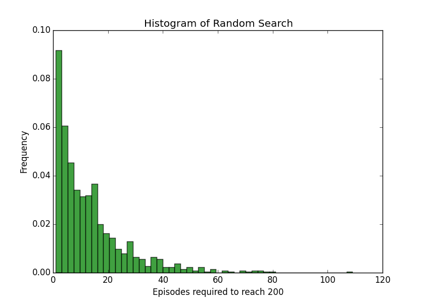
I ran the random search method 1,000 times, keeping track of how many episodes it took until the agent kept the pole up for 200 timesteps. On average, it took 13.53 episodes.
Hill-Climbing
Another method of choosing weights is the hill-climbing algorithm. We start with some randomly chosen initial weights. Every episode, add some noise to the weights, and keep the new weights if the agent improves.
noise_scaling = 0.1
parameters = np.random.rand(4) * 2 - 1
bestreward = 0
for _ in xrange(10000):
    newparams = parameters + (np.random.rand(4) * 2 - 1)*noise_scaling
    reward = 0
    run = run_episode(env,newparams)
    if reward > bestreward:
        bestreward = reward
        parameters = newparams
        if reward == 200:
            break
The idea here is to gradually improve the weights, rather than keep jumping around and hopefully finding some combination that works. If noise_scaling is high enough in comparison to the current weights, this algorithm is essentially the same as random search.
As usual, this algorithm has its pros and cons. If the range of weights that successfully solve the problem is small, hill climbing can iteratively move closer and closer while random search may take a long time jumping around until it finds it.
However, if the weights are initialized badly, adding noise may have no effect on how well the agent performs, causing it to get stuck.
To visualize this, let's pretend we only had one observation and one weight. Performing random search might look something like this.
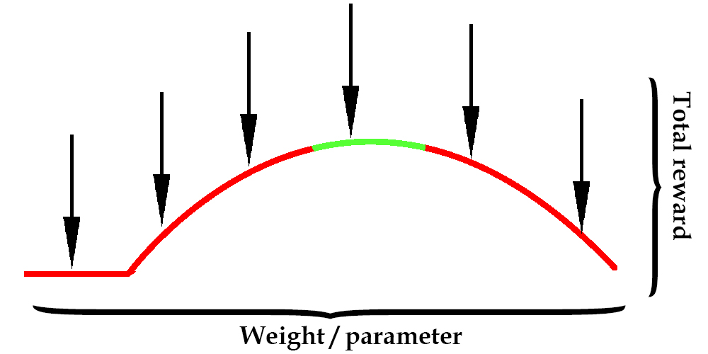
In the image above, the x-axis represents the value of the weight from -1 to 1. The curve represents how much reward the agent gets for using that weight, and the green represents when the reward was high enough to solve the environment (balance for 200 timesteps).
An arrow represents a random guess as to where the optimal weight might be. With enough guesses, the agent will eventually try a weight in the green zone and be successful.
How does this change with hill climbing?
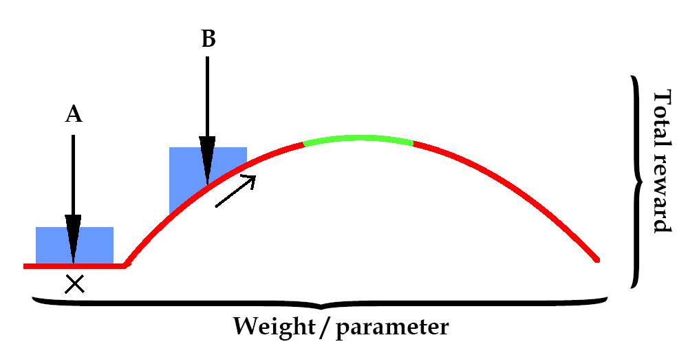
Here, an arrow represents the value that weights are initialized at. The blue region is noise that is added at every iteration.
If the weight starts at arrow B, then hill-climbing can try other weights near arrow B until it finds one that improves the reward. This can continue until the weight is in the green zone.
However, arrow A has a problem. If the weight is initialized at a location where changing it slightly gives no improvement at all, the hill climbing is stuck and won't find a good answer.
It turns out that in CartPole, there are many initializations that get stuck.
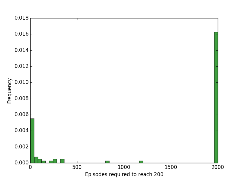
More than half of the trials got stuck and couldn't improve (the bar on the right). However, of the trials that reach a solution, it took an average of 7.43 episodes to do so, less than random search.
A possible fix to this problem would be to slightly increase the noise_factor every iteration that the agent does not improve, and eventually reach a set of weights that improves the reward.
Another change that may improve accuracy is to replace
reward = run_episode(env,parameters)
with
reward = 0
for _ in xrange(episodes_per_update):
    run = run_episode(env,newparams)
    reward += run
Instead of only running one episode to measure how good a set of weights is, we run it multiple times and sum up the rewards. Although it might take longer to evaluate, this decreases variance and results in a more accurate measurement of whether one set of weights performs better.
Policy Gradient
The next method is a little more complicated than needed to solve the CartPole environment. When possible, simple methods such as random search and hill climbing are better to start with. However, it's a good concept to learn and performs better in environments with lots of states or actions.
In order to implement a policy gradient, we need a policy that can change little by little. In practice, this means switching from an absolute limit (move left if the total is < 0, otherwise move right) to probabilities. This changes our agent from a deterministic to a stochastic (random) policy.
Instead of only having one linear combination, we have two: one for each possible action. Passing these two values through a softmax function gives the probabilities of taking the respective actions, given a set of observations. This also generalizes to multiple actions, unlike the threshold we were using before.
Since we're going be computing gradients, it's time to bust out Tensorflow.
def policy_gradient():
    params = tf.get_variable("policy_parameters",[4,2])
    state = tf.placeholder("float",[None,4])
    linear = tf.matmul(state,params)
    probabilities = tf.nn.softmax(linear)
We also need a way to change the policy, increasing the probability of taking a certain action given a certain state.
Here's a crude implementation of an optimizer that allows us to incrementally update our policy. The vector actions is a one-hot vector, with a one at the action we want to increase the probability of.
def policy_gradient():
    params = tf.get_variable("policy_parameters",[4,2])
    state = tf.placeholder("float",[None,4])
    actions = tf.placeholder("float",[None,2])
    linear = tf.matmul(state,params)
    probabilities = tf.nn.softmax(linear)
    good_probabilities = tf.reduce_sum(tf.mul(probabilities, actions),reduction_indices=[1])
    # maximize the log probability
    log_probabilities = tf.log(good_probabilities)
    loss = -tf.reduce_sum(log_probabilities)
    optimizer = tf.train.AdamOptimizer(0.01).minimize(loss)
So we know how to update our policy to prefer certain actions. If we knew exactly what the perfect to move in every state was, we could just continously perform supervised learning and the problem would be solved. Unfortunately, we don't have some magic oracle that knows all the right moves.
We want to know how good it is to take some action from some state. Thankfully, we do have some measure of success that we can make decisions based on: the return, or total reward from that state onwards.
We're trying to determine the best action for a state, so the first thing we need is a baseline to compare from. We a define some value for each state, that contains the average return starting from that state. In this example, we'll use a 1 hidden layer neural network.
def value_gradient():
    # sess.run(calculated) to calculate value of state
    state = tf.placeholder("float",[None,4])
    w1 = tf.get_variable("w1",[4,10])
    b1 = tf.get_variable("b1",[10])
    h1 = tf.nn.relu(tf.matmul(state,w1) + b1)
    w2 = tf.get_variable("w2",[10,1])
    b2 = tf.get_variable("b2",[1])
    calculated = tf.matmul(h1,w2) + b2

    # sess.run(optimizer) to update the value of a state
    newvals = tf.placeholder("float",[None,1])
    diffs = calculated - newvals
    loss = tf.nn.l2_loss(diffs)
    optimizer = tf.train.AdamOptimizer(0.1).minimize(loss)
In order to train this network, we first need to run some episodes to gather data. This is pretty similar to the loop in random-search or hill climbing, except we want to record transitions for each step, containing what action we took from what state, and what reward we got for it.
# tensorflow operations to compute probabilties for each action, given a state
pl_probabilities, pl_state = policy_gradient()
observation = env.reset()
actions = []
transitions = []
for _ in xrange(200):
    # calculate policy
    obs_vector = np.expand_dims(observation, axis=0)
    probs = sess.run(pl_probabilities,feed_dict={pl_state: obs_vector})
    action = 0 if random.uniform(0,1) < probs[0][0] else 1
    # record the transition
    states.append(observation)
    actionblank = np.zeros(2)
    actionblank[action] = 1
    actions.append(actionblank)
    # take the action in the environment
    old_observation = observation
    observation, reward, done, info = env.step(action)
    transitions.append((old_observation, action, reward))
    totalreward += reward

    if done:
        break
Next, we compute the return of each transition, and update the neural network to reflect this. We don't care about the specific action we took from each state, only what the average return for the state over all actions is.
vl_calculated, vl_state, vl_newvals, vl_optimizer = value_gradient()
update_vals = []
for index, trans in enumerate(transitions):
    obs, action, reward = trans
    # calculate discounted monte-carlo return
    future_reward = 0
    future_transitions = len(transitions) - index
    decrease = 1
    for index2 in xrange(future_transitions):
        future_reward += transitions[(index2) + index][2] * decrease
        decrease = decrease * 0.97
    update_vals.append(future_reward)
update_vals_vector = np.expand_dims(update_vals, axis=1)
sess.run(vl_optimizer, feed_dict={vl_state: states, vl_newvals: update_vals_vector})
If we let this run for a couple hundred episodes, the value of each state is represented pretty accurately. The decrease factor puts more of an emphasis on short-term reward rather than long-term reward. This introduces a little bias but can reduce variance by a lot, especially in the case of outliers, such as a lucky episode that lasted for 100 timeframes from a state that normally lasted only 30.
How can we use the newly found values of states in order to update our policy to reflect it? Obviously, we want to favor actions that return a total reward greater than the average of that state. We call this error between the actual return and the average an advantage. As it turns out, we can just plug in the advantage as a scale, and update our policy accordingly.
for index, trans in enumerate(transitions):
    obs, action, reward = trans
    # [not shown: the value function update from above]
    obs_vector = np.expand_dims(obs, axis=0)
    currentval = sess.run(vl_calculated,feed_dict={vl_state: obs_vector})[0][0]
    advantages.append(future_reward - currentval)
advantages_vector = np.expand_dims(advantages, axis=1)
sess.run(pl_optimizer, feed_dict={pl_state: states, pl_advantages: advantages_vector, pl_actions: actions})
This requires a slight change in our policy update: we add in a scaling factor for a given update. If a certain action results in a return of 150, while the state average is 60, we want to increase its probability more than an action with a return of 70 and a state average of 65. Furthermore, if the return for an action is 30 while the state is average is 40, we have a negative advantage, and instead decrease the probability.
def policy_gradient():
    params = tf.get_variable("policy_parameters",[4,2])
    state = tf.placeholder("float",[None,4])
    actions = tf.placeholder("float",[None,2])
    advantages = tf.placeholder("float",[None,1])
    linear = tf.matmul(state,params)
    probabilities = tf.nn.softmax(linear)
    good_probabilities = tf.reduce_sum(tf.mul(probabilities, actions),reduction_indices=[1])
    # maximize the log probability
    log_probabilities = tf.log(good_probabilities)
    # insert the elementwise multiplication by advantages
    eligibility = log_probabilities * advantages
    loss = -tf.reduce_sum(eligibility)
    optimizer = tf.train.AdamOptimizer(0.01).minimize(loss)
How well does our policy gradient perform on CartPole?
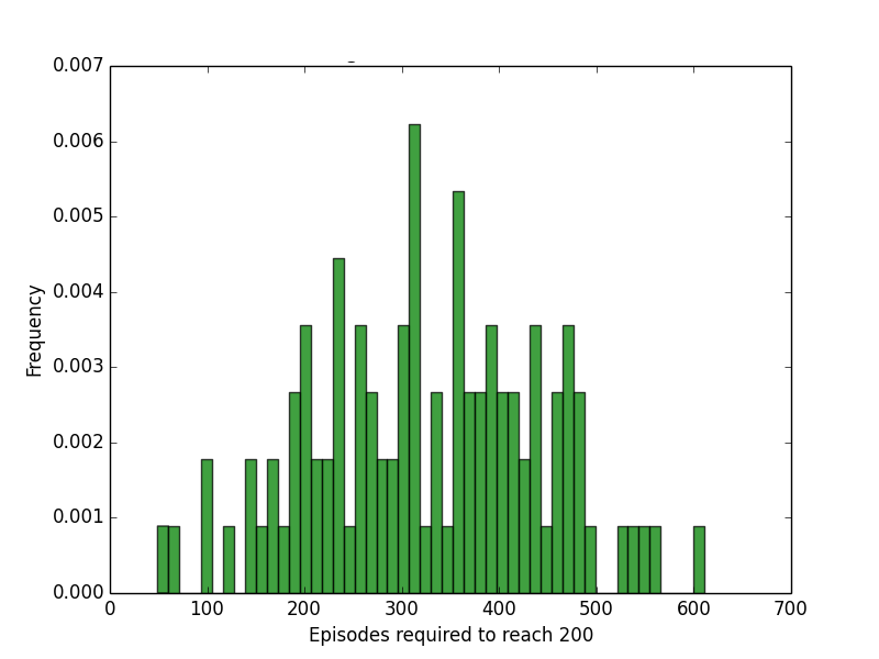
Turns out, it's not very fast. Compared to random search and hill climbing, policy gradient takes much longer to solve CartPole.
This is partly due to having to learn a value function first, before the agent can make any solid assumptions as to which actions are better. While the first two methods can start improving right off the bat, the policy gradient needs to collect data on how to improve first.
However, this ensures that the updates are always making some form of improvement. In environments with much higher dimensional state spaces, the previous methods get much less efficient, as the probability of improving when adjusting randomly is small. A policy gradient ensures the agent is always heading toward some kind of optimum.
Since we always follow the gradient, our weights will always be changing and we doesn't get stuck in bad initializations such as in hill climbing. It also can improve on an already good solution even further, which random search cannot do.
In the end, simple methods are almost always better when dealing with simple problems. For more complicated environments, a policy gradient allows our agent to perform more consistent updates and gradually improve.
The code for these methods is available on my Github