If you look through the results on the OpenAI gym, you'll notice an algorithm that consistently performs well over a wide variety of tasks: Trust Region Policy Optimization, or TRPO for short.
However, the algorithm does take quite a bit of time to converge on these environments. In this post, I'll go over the methods and thinking behind using both parallelization and parameter adaptation for a more efficient algorithm, following this request for research.
What is Trust Region Policy Optimization?
The first thing we need to understand: what exactly is TRPO? The paper on the subject goes into more detail, but essentially, it's a policy gradient method with a fancy gradient optimizer.
Rather than updating the policy's parameters directly in accordance to its gradient, we use the natural gradient. This limits the KL divergence between our new and old policy, instead of limiting the change in our parameter values (stepsize in traditional gradient descent). For more details on the natural gradient, check out this post.
Other than the special gradient function, TRPO behaves as a standard policy gradient method. We run through the environment many times and calculate a value function that estimates the total future reward of being in a certain state. Then, we update the our agent's policy as to increase the probability of entering states with greater predicted value. Repeat this many times and (hopefully) the agent will learn the optimal policy!
How can it be improved?
Here's the big question. How can we make it faster? To get some hints as to where to start, I ran a trial on Reacher-v1 and measured how long the agent spent on each phase.
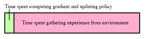
Clearly, it's taking a long time gathering experience! This makes sense: we're collecting 20,000 timesteps of data before every update, and each timestep requires the computer to not only simulate the environment, but run through the policy as well.
We now know which portion requires improvement, but how do we go about doing that?
Parallelization
Computers these days don't run only on a single thread; multiple things can be happening at the same time. Of course, how many threads we can use is limited by the number of cores our CPU has.
We can take advantage of this by splitting up the work of gathering experience. Instead of having a single actor run the environment 20,000 times, we can have multiple actors run only 6,000 times each.
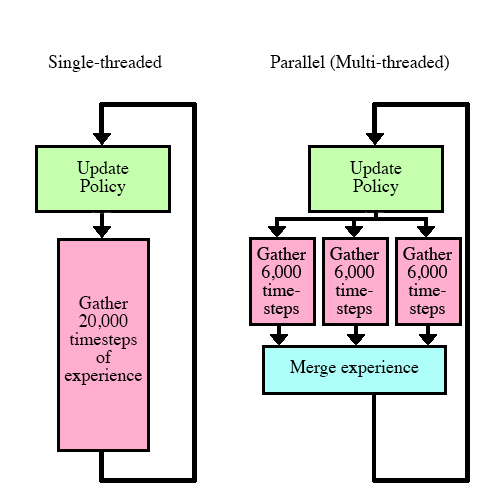
Single vs Multiple actor setup
This is where the Monte Carlo sampling portion of TRPO comes in handy.
In some reinforcement learning algorithms, such as one-step Q learning, we take one step in the environment, update the policy, and repeat. This often involves having another neural network represent the value function, and training it in addition to the policy.
With Monte Carlo, we record 20,000 timesteps with the exact same policy before every update, and recalculate the value function every time. This is more stable, as a neural network doesn't always represent the value function accurately, especially in earlier iterations.
Running through all the timesteps with the same policy is key in parallelization: in python multiprocessing, separate threads can't communicate with each other until the task has been finished.
If we were using, say, the one-step Q learning method, each actor would have to keep its own independent policy and update it after every timestep. Then they would average their policies every few hundred updates. This might lead to suboptimal results that differ from a single-threaded implementation.
However, in our case, we don't update the policy until all the threads have finished. The data we collect is exactly the same as if we were single-threaded!
How well does it work?
I ran both a single-threaded and a 5-threaded version on a 5 core CPU to see how they compared.
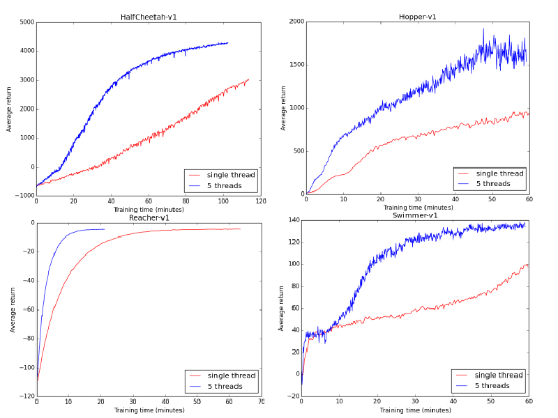
In every case, the parallel implementation was faster in terms of wall-clock time by a major factor. In a completely ideal situation, the speedup would have been 5x, plus or minus some time taken to merge the experience and compute a gradient update.
A potential method to improve even further is to simply add more threads. I ran trials using varying amounts of threads on Reacher-v1, an environment proven to be stable.
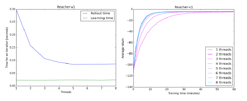
As it turns out, there are some big diminishing returns on just blindly adding threads. Using two threads reduces the time taken to collect data by 50%, three by 66%, and from four onwards we start to flatline.
The most likely reason is that we reached a hardware limit. My computer doesn't have infinite parallel computing power, it only has 5 cores. If we had used a machine with, for example, 16 cores, I'm sure the speeds would go down even lower before leveling off.
Finally, there will always be a bit of overhead to running the learner, regardless of how fast we can collect the data. The green line in the first graph shows the time taken to actually run gradient computation and create a new policy. The 5 threaded version still takes a majority of the time collecting data, but as the times go lower, we would have to start thinking about optimizing other parts of the learning process.
Hyperparameter adaptation
So we've got a parallel method that speeds up our data collection significantly. However, we're still using this data inefficiently. For every update, we collect 20,000 timesteps worth of experience, use it to make one small update, then discard it. Is there a way to improve this?
One potential option is to decrease the number of timesteps we experience between each update. We're only using this experience to estimate a value function, and we can potentially do just fine with less samples. I ran some tests on Reacher to see how reducing the timesteps/update affected the learning curve.
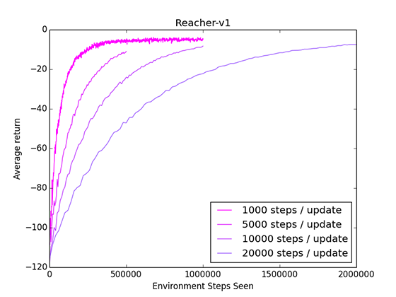
It works! We can get faster convergence by reducing the steps/update. However, there are downsides as well. Using less experience results in a less accurate value function estimate, which in turn results in a less accurate policy update.
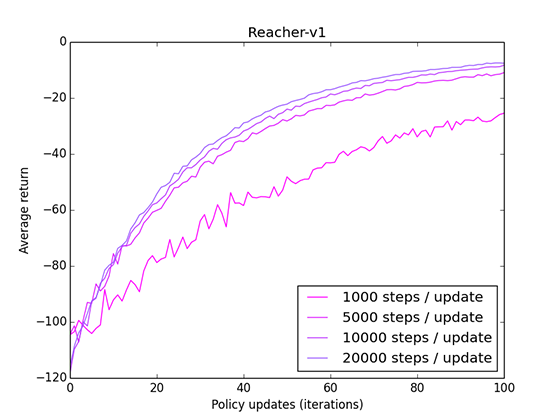
When comparing by the number of updates, rather than number of timesteps, we can see that using 1000 steps/update results in a noisy and sub-optimal update.
However, at least for this environment, we can converge faster using many less-accurate updates, rather than a few accurate but experience-intensive updates.
In a similar vein, we can also adjust the maximum KL parameter.
In TRPO, we update the policy using a natural gradient. Rather than having a stepsize to limit our change, as in traditional gradient updates, we have a maximum KL that the policy is allowed to diverge.
Conceptually, we can think of stepsize and max KL as the same kind of setting: how much we want to change the policy.
Of course, we always want to be taking the biggest update we can, assuming the gradient direction is accurate and not overshooting the optimal policy. Again, I ran a test to see how the agent performed with a bigger max KL parameter.
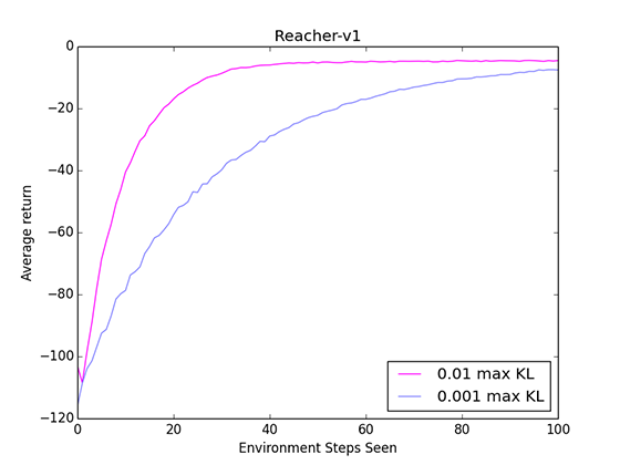
A greater max KL means we converge faster! Of course, Reacher is a simpler environment where the policy is usually updating in the same direction. The same cannot be said for every environment. Using too big of a max KL would not only have a chance to overshoot the optimal policy, but it would also make it harder to make the small and precise updates required when nearing convergence.
So what should we change the parameters to?
Both the steps/update and max KL parameters have the potential to increase efficiency. However, they both have downsides that can lead to bad convergence.
The problem here is that the "perfect" parameters are different for each environment. For example, in a simple setting such as Reacher, updating only based on 1,000 steps may work fine. In a more complicated environment such as Swimmer, having so few steps wouldn't be enough to update accurately.
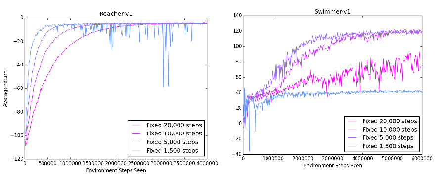
The blue lines show how having only a few steps/update leads to unstable results. In Reacher, the effect is not as pronounced: we still perform well, just with spikes of bad performance. In Swimmer, we really get the worst case. There is so little data that the policy can barely improve at all, keeping the average reward down near 40.
In both environments, 5,000 steps/update was the optimal parameter, with both high speeds and very little variation. In other environments, the optimal parameter may very well be something completely different. However, it is impractical to run a trial on every environment that for the best parameters: we want a method that can work across everything.
The adaptive method
To find a solution, I tried to think about the problem from the perspective of what I would do if I could change these parameters in real-time.
If the total average reward is steadily rising, that means the policy is updating in the right direction. I would increase the KL, allowing the policy to make bigger updates, as they have proven to be accurate. I would also decrease the steps/update, as we know that the current steps/update leads to an accurate update, and we should squeeze the most value out of our experience.
On the other hand, if the policy was stuck and not improving, I would decrease the KL, as smaller steps would prevent overshooting the optimal policy. I would also increase the steps/update, in an attempt to get a more accurate update.
The adaptive method is simply these two rules, built-in to the agent itself. Every update, we compare the total reward to that of the last update. If we have improved, we can then reduce steps/update, and try for a more efficient but less accurate update. If we're stuck, we can increase steps/update, and sacrifice some efficiency for more accurate updates.
We can do the same with max KL, although we'd have to reverse the change (increase max KL when decreasing steps/update).
One thing to note is that increasing KL and decreasing steps/update essentially accomplish similar goals, and it may be redundant to do both.
How well did it work?
I tested three kinds of adaptive methods: adapt the steps/update, adapt the max KL, or adapt both. For comparison, I plotted the reward curves using both the original parameters, and the optimal parameters for that environment using a brute-force search.
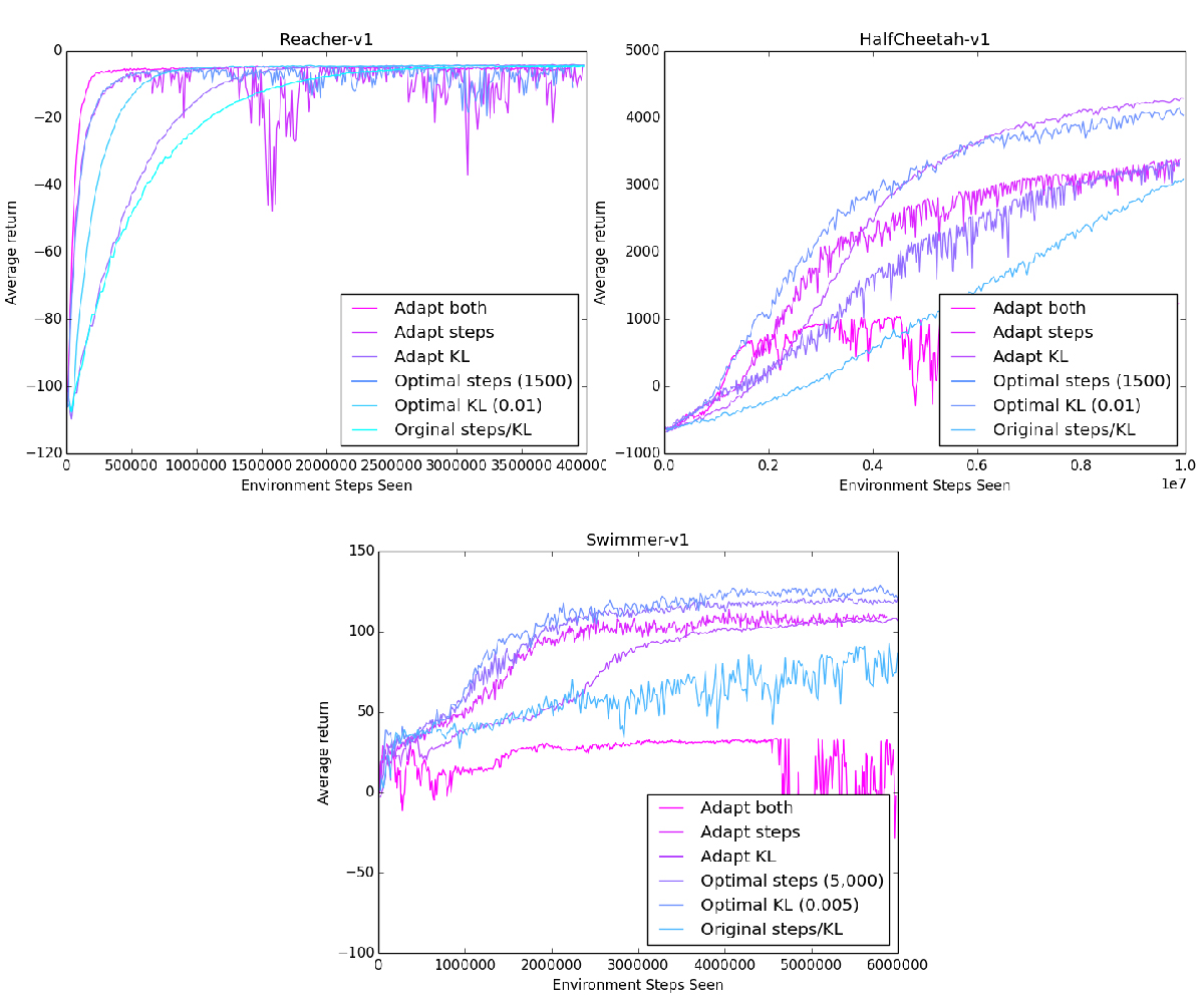
While we don't reach the performance of the optimal parameters on every environment, we definitely outperformed the original fixed parameters!
Interesting to note is that there is no definite best parameter to adapt. In Reacher and Swimmer, adapting steps/update performed better, while in HalfCheetah, adapting the max KL performed better.
We can also take a look at the trial where both steps/update and max KL were adapted. In Reacher, this extreme push for efficiency worked well, outperforming every other method.
However, in the other two environments, adapting both parameters fails horribly. We can't even pass the performance of the original parameters, instead we get stuck at a low reward with no signs of improvement.
After running the trials again, I realized the potential problem. The low steps/update and high max KL led the agent to make big updates in completely inaccurate directions. This put the policy in a state where a single update wouldn't make any improvement. The agent would then be stuck, constantly increasing and decreasing the steps/update due to random variation, rather than based on its performance.
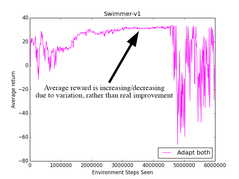
Essentially, when the average reward was staying relatively constant, we weren't changing the parameters at all. This is bad! If we're not improving, we want to be increasing the steps/update so we have a more accurate gradient!
How could this be fixed? I implemented an improvement margin required in order for the agent to decrease the steps/update.
For example, we could impose a margin of 5%, meaning the agent would have to improve by 5% in order to decrease its steps/update. If the agent isn't improving by at least 5%, we'll increase the steps/update.
This ensures that when the average reward is neither moving up or down, it won't get stuck adapting its parameters back and forth, as described earlier. Instead, the situation is considered under the 5% margin, so the agent would increase the steps/update for better accuracy.
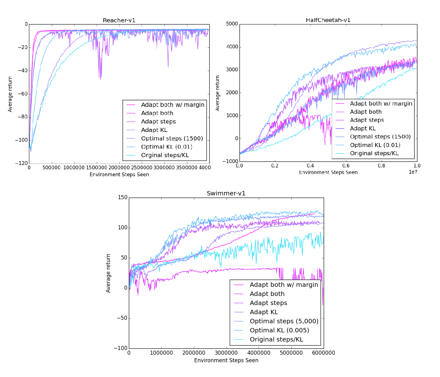
With pleasant surprise, the margin worked very well! The trials that adapted both KL and steps no longer diverged badly, instead performing on a level consistently near the top.
The performance on Reacher also took no hits: in the simple environment, the adaptive-margin was still able to focus on full efficiency and improve quickly.
Finally, one last thing to note is we don't want to adapt every single update. Rather, we sum up the rewards in the past 10 updates, and compare it to the 10 before that. This reduces variation and gets us a better picture of how the policy is improving.
Conclusion and next steps
Utilizing parallelization and hyperparameter adaptation, we were able to take the Trust Region Policy Optimization algorithm and increase its speed to a major extent.
I'm currently running more trials for Humanoid, a more complex environment, to see how the adaptive method performs when the optimal parameters change throughout learning.
I'll probably also upload some of these results to gym, and see how they compare to others.
Big thanks to John Schulman for helping me with many things and providing feedback!
Also, thanks to Danijar Hafner for helping a lot as well; we are currently working to update this preliminary paper to include the hyperparameter adaptation.
The code for this post is available on my Github.