Successor Representations Explained

Note: We're going to conflate terminology for value-functions and Q-functions. In general the Q-function $Q(s,a)$ is just an action-conditioned version of the value function $V(s)$.

Successor Representations

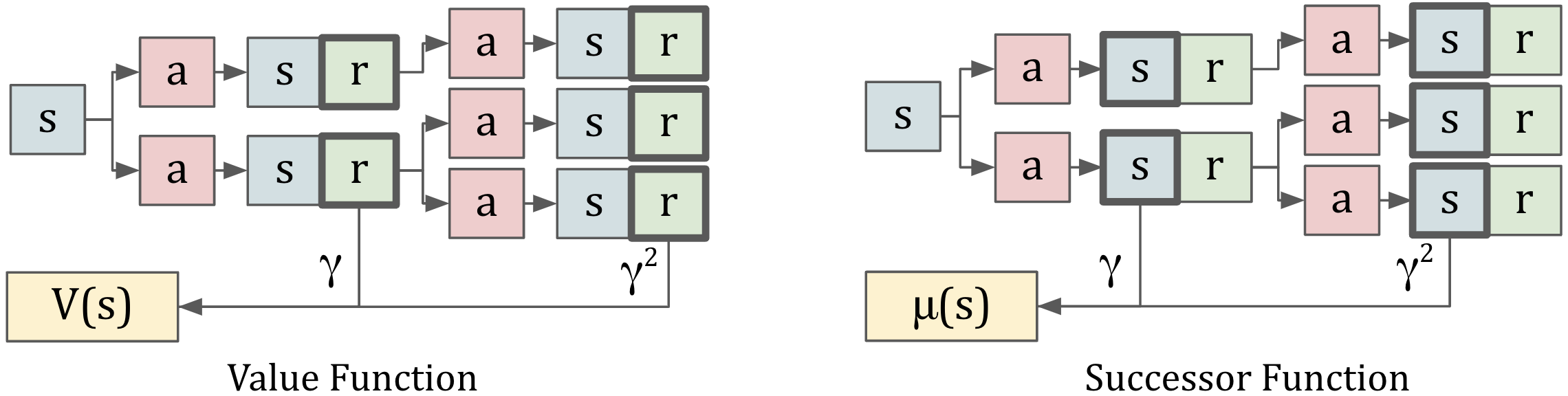
Let's consider a classic temporal difference method -- estimating the value function. The value of a state is the expected discounted sum of future rewards, starting from that state. Notably, temporal difference methods give us a nice recursive form of the value function.

$V(s) = r + \gamma E_{p(s'|s)}[V(s')]$

Learning a value function is helpful because it lets us reason about future behaviors, from a single function call. What if we could do this not over reward, but over states themselves?

Successor representations are an application of temporal difference learning, where we predict expected state occupancy. If I follow my policy, discounted into the future, what states will I be in?

This is easily understandable in a MDP with discrete states. Let's say I start out in state A. After one timestep, I transition into a probability distribution over A,B,C. Each path then leads to a distribution for t=2, then t=3, etc. Now, we'll combine all of these distributions as a weighted average.

$\mu(s^*|s) = (1-y)p(s'|s) + \gamma E_{p(s'|s)} \mu(s^*|s')$

Looks similar to the value function, doesn't it. Successor representations follow the same structure as the value function, but we're accumulating state probabilities rather than expected reward.

Gamma Models

In more recent methods, we use deep neural networks to learn the successor representation. Gamma models attempt to a learn an action-conditioned successor function $\mu(s^*|s,a)$. Notably, $\mu$ is a generative model and can handle both continuous and discrete settings. That means we can learn $\mu(s^*|s,a)$ using our favorite generative-modelling methods. The paper uses GANs and normalizing flows.

This interpretation gives us some nice properties:

• If our reward function is $\delta(s = s^*)$ (i.e. sparse reward at some goal state), then the value of any state is equivalent to evaluating the gamma-model at $\mu(s^*|s,a)$. The value function of a sparse reward is equal to the probability that the policy occupies that state.
• We can extract the value function for arbitrary reward functions as well. It involves a sum over trajectories sampled from the policy:
  • $Q(s,a) = \sum \mu(s^*|s,a) \; r(s^*)$
• If we set $\gamma=0$, then the gamma model is actually a one-step world model. In this case, $\mu(s^*|s,a) = p(s'|s,a)$ and we're simply modelling the environment's transition dynamics.

Forward-Backward Models

This next work describes FB models, an extension of successor representations that lets us extract optimal policies for any reward function.

Above, we showed we can extract any Q(s,a), given a reward function r(s) and $\mu(s^*|s,a)$. In continuous space, we need to sum over trajectories to compute $Q_r(s,a) = \sum \mu(s^*|s,a) \; r(s^*)$. In discrete space, $\mu(s^*|s,a)$ can directly output a vector over $s$, and we can compute Q with a matrix multiplication $Q(s,a) = \mu(s,a)^Tr$. Moving forward, we'll assume we are in the continuous setting.

A key insight about value-functions and successor-functions is that they are policy-dependent. Depending on the policy, the distribution of future (reward/states) will change. Assuming we had some representation of a policy $z$, we could train a policy-conditioned successor function $\mu(s^*|s,a,z)$. We can further decompose $\mu$ into the policy-dependent and -independent parts, F and B. $\mu(s^*|s,a,z) = F(s,a,z)^TB(s^*)$.

Let's take a look at that decomposition in detail. The original $\mu$ is a neural-network with inputs $(s^*,s,a,z)$. It returns a scalar of the probability of being in state $s^*$. In the decomposition, F is a network with inputs (s,a,z) and output (d). B is a network with inputs ($s^*$), outputting a vector (d,1). A final dot product reduces these vectors into a scalar. One way to think about these representations is: F(s,a,z) calculates a set of expected future features when following policy $z$. B(d,s*) then calculates how those features map back to real states.

Now, how do we find $\pi_z$ that is optimal for every reward function? Well, we need a way to learn a function z(r). The trick here is we can choose this function, so let's be smart about it. Let's define z(r) = $\sum B(s^*) \; r(s^*)$. Some derivations:
- Remember that the Q-function for any $r$ was $Q_r(s,a) = \sum \mu(s^*|s,a) \; r(s^*)$.
- Also, we decomposed $\mu(s^*|s,a,z) = F(s,a,z)^TB(s^*)$.
- The optimal Q is thus $\sum F(s,a,z)^TB(s^*) \; r(s^*)$ = $F(s,a,z)^T \sum B(s^*) \; r(s^*)$ .
- Based on $z(r) = \sum B(s^*) \; r(s^*)$, we get $Q(s,a,z) = F(s,a,z)^Tz$

Notably, the reward term has disappeared! Let's interpret. The $z$ vector here is playing two roles. First, it serves a policy representation that is given to F -- it contains information about the behavior of $\pi_z$. Second, it serves as a feature-reward mapping -- it describes how much reward to assign to each successor feature.

The F and B networks are trained without any reward-function knowledge. We'll do the same thing as in previous works. We update $\mu = FB$ through a Bellman update. Remember that $\pi(s',z) = \text{argmax} \; F(s,a,z)^Tz$, and $\mu = F(s,a,z)^TB(s^*)$.

$\mu(s^*|s,a,z) = \delta(s=s^*) + \gamma E_{p(s'|s,a)} \mu(s^*|s',\pi(s',z),z)$
$F(s,a,z)^TB(s^*) = \delta(s=s^*) + \gamma E_{p(s'|s,a)} F(s,\text{argmax} \; F(s',a,z)^Tz,z)^TB(s^*)$

You'll notice that in addition to trajectories, this update is conditioned on $z$. Since we don't know $z$ ahead of time, we just need to guess -- we'll generate random $z$ vectors from a Gaussian distribution.

Test Time. Once we've learned F and B, extracting the optimal policy is simple. We'll calculate $z = \sum B(s^*) \; r(s^*)$. That gives us our Q-function $Q(s,a,z) = F(s,a,z)^Tz$, which we can act greedily over.