Variational Information Bottleneck Explained

Let's take a look at neural networks from the perspective of information theory. We'll be following along with the paper Deep Variational Information Bottleneck (Alemi et al. 2016).

Given a dataset of inputs $X$ and outputs $Y$, let's define some intermediate representation $Z$. A good analogy here is that $Z$ is the features of a neural network layer. The standard objective is to run gradient descent so to predict $Y$ from $X$. But that setup doesn't naturally give us good representations. What if we could write an objective over $Z$?

One thing we can say is that $Z$ should tell us about the output $Y$. We want to maximize the mutual information $I(Z,Y)$. This objective makes natural sense, we don't want to lose any important information.

Another thing we could say is that we should minimize the information passing through $Z$. The mutual info $I(Z,X)$ should be minimized. We call this the information bottleneck. Basically, $Z$ should keep relevant information about $Y$, but discard the rest of $X$.

The tricky thing is that mutual information is hard to measure. The definition for mutual information involves optimal encoding and decoding. But we don't have those optimal functions. Instead, we need to approximate them using variational inference.

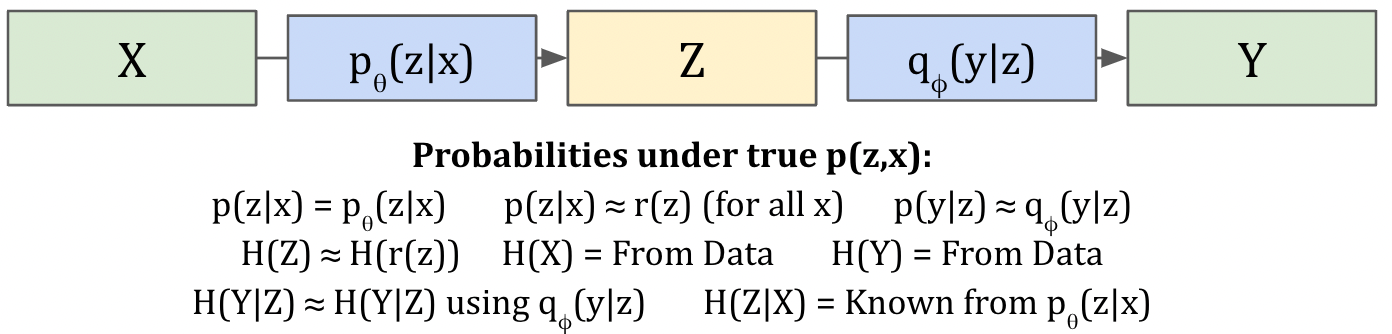
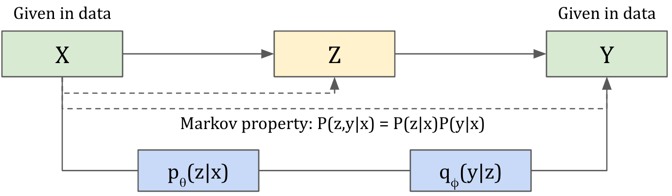
Let's start by stating a few assumptions. First we'll assume that X,Y,Z adhere to the Markov chain (Y - X - Z). This setup guarantees that P(Z|X) = P(Z|X,Y) and P(Y|X) = P(Y|X,Z). In other words, Y and Z are independent given X. We'll also assume that we're training a neural network to model p(z|x).

Information Bottleneck Objective

Here's our main information bottleneck objective ($\beta$ determines the "strength" of the bottleneck):

$I(Z,Y) - \beta I(Z,X)$.

We'll break it down piece by piece. Looking at the first term:

$I(Z,Y) = H(Y) - H(Y|Z)$
$I(Z,Y) = H(Y) + \int p(y,z) \; log \; p(y|z)$ (Definition of conditional entropy.)

The H(Y) term is easy, because it's a constant. We can't change the output distribution because it's defined by the data.

The second conditional term is trickier. Unfortunately, p(y|z) isn't tractable. We don't have that model. So we'll need to approximate it by introducing a second neural network, q(y|z). This is the variational approximation trick.

The key to this trick is recognizing the relationship between $\int p(y,z) \; log \; p(y|z)$ and KL divergence. KL divergence is always positive, so $\int p(y,z) \; log \; p(y|z) \geq \int p(y,z) \; log \; q(y|z)$. That means we can plugin q(y|z) instead of p(y|z) and get a lower bound. Another way to interpret this trick is: H(Y|Z) is the lowest entropy we can achieve using $Z$ in the optimal way. If we use $Z$ in a sub-optimal way, that's an upper bound on the true entropy. The overall term is lower-bounded because we subtract H(Y|Z).

Because of the Markovian assumption above, we can break down p(y,z) into p(y|x)p(z|x). This version is easier to sample from.

Let's look at the second term now. We will use a similar decomposition.

$I(Z,X) = H(Z) - H(Z|X)$
$I(Z,X) = -\int p(z) \; log \; p(z) + \int p(x,z) \; log \; p(z|x)$

This time, the second term is the one that is simple. We have the model p(z|x), so we can calculate the log-probability by running the model forward. The p(z) term is tricky. It's not possible to compute p(z) directly, so we approximate it with r(z). The same KL-divergence trick makes this an upper bound to H(Z).

Putting everything together, the information bottleneck term becomes:

$I(Z,Y) - \beta I(Z,X) \geq \int p(x)p(y|x)p(z|x) \; log \; q(y|z) - \beta \int p(x)p(z|x) log \; \dfrac{p(z|x)}{r(z)}$

It's simpler than it looks. We can compute an unbiased gradient of the above term using sampling. Once we sample $x \sim X$, we can calculate p(y|x) and p(z|x) by running the model forward. The second term is actually a KL divergence between p(z|x) and r(z), which can be computed analytically if we assume both are Gaussian.

Thus the objective function can be written as:

$\text{min}_\theta \; E[-log \; q_\phi(y|p_\theta(z,x)) + \beta \; KL(p_\theta(z|x) || r(z))]$

Intuitions

Let's go over some intuitions about the above formula.

1. The first part is equivalent to maximizing mutual information between Y and Z. Why is this equivalent? Mutual information can be written as $H(Y) - H(Y,Z)$. The first term is fixed. The second term asks "what is the best predictor of Y we can get, using Z"? We're training the network $q_\phi$ to do precisely this objective.

2. The second part is equivalent to minimizing mutual information between $Z$ and $X$. Why? Because no matter which $x$ is sampled, we want the posterior distribution $p_\theta(z|x)$ to look like $r(z)$. In other words, if this term is minimized to zero, then p(z|x) would be the same for every $x$. This is the "bottleneck" term.

3. The variational information bottleneck shares a lot of similarities with the variational auto-encoder. We can view the auto-encoder as a special case of the information bottleneck, where Y=X. In fact, the VAE objective $\text{min}_\theta \; E[-log \; q_\phi(x|p_\theta(z,x)) + KL(p_\theta(z|x) || r(z))]$ is equivalent to what we derived above, if y=x and $\beta=1$.

   If we set X=Y, one could ask, isn't it weird to maximize $I(Z,X) - I(Z,X)$? It's just zero. The answer is that we're optimizing different approximations to those two terms. The first term is the recreation objective, which optimizes a bound on H(X|Z). The second is the prior-matching objective, which optimizes the true H(Z|X) and a bound on H(Z).

4. What extra networks are needed to implement the variational information bottleneck? Nothing, really. In the end, we're splitting y=f(x) into two networks, p(z|x) and q(y|z). And we're putting a bottleneck on $z$ via an auxiliary objective that it should match a constant prior r(z).