A few months ago I attempted to understand the natural gradient, and wrote a post to help organize what I knew. Unfortunately there was too little detail and all I really understood was a "black box" version of the natural gradient: what it did, not how it worked on the inside.
In this post, I'm going to go into detail about how the natural gradient works, explained at a level for people with only a small understanding of the linear algebra and statistical methods.
What is the natural gradient?
First off, we must understand standard gradient descent.
Let's say we have a neural network, parameterized by some vector of parameters. We want to adjust the parameters of this network, so the output of our network changes in some way. In most cases, we will have a loss function that tells our network how it's output should change.
Using backpropagation, we calculate the derivatives of each parameter with respect to our loss function. These derivatives represent the direction in which we can update our parameters to get the biggest change in our loss function, and is known as the gradient.
We can then adjust the parameters in the direction of the gradient, by a small distance, in order to train our network.
A slight problem appears in how we define "a small distance".
In standard gradient descent, distance means Euclidean distance in the parameter space.
#for example, with two parameters (a, b)
distance = sqrt(a^2 + b^2)
However, defining "distance" in terms of how much our parameters is adjusted isn't always correct. To visualize this, let's take a look at two pairs of gaussian distributions.
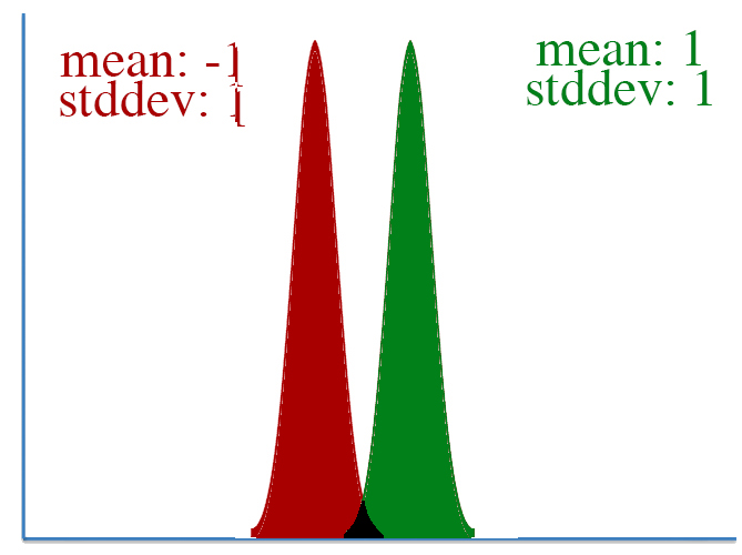
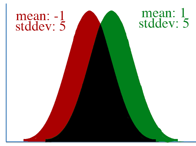
In both distributions, the mean is changed from -1 to 1, a distance of two. However, it's clear that the first distribution changed far more than the second.
This leads to a key insight: our gradient measures how much our output is affected by changing a parameter. However, this affect on the output must be seen in context: a shift of +2 in the first distribution means a lot more than a shift of +2 in the second one.
What the natural gradient does is redefine the "small distance" we update our parameters by. Not all parameters are equal. Rather than treating a change in every parameter equally, we need to scale each parameter's change according to how much it affects our network's entire output distribution.
How do we do that?
First off, let's define a new form of distance, that corresponds to distance based on KL divergence, a measure of how much our new distribution differs from our old one.
We do this by defining a metric matrix, which allows us to calculate the distance of a vector according to some custom measurement.
For a network with 5 parameters, our metric matrix is 5x5. To compute the distance of a change in parameters delta using metric, we use the following:
totaldistance = 0
for i in xrange(5):
    for j in xrange(5):
        totaldistance += delta[i] * delta[i] * metric[i][j]
If our metric matrix is the identity matrix, the distance is the same as if we just used Euclidean distance.
However, most of the time our metric won't be the identity matrix. Having a metric allows our measurement of distance to account for relationships between the various parameters.
As it turns out, we can use the Fisher Information Matrix as a metric, and it will measure the distance of delta in terms of KL divergence.
The Fisher Information Matrix is the second derivative of the KL divergence of our network with itself. For more information on why, see this article.
The concept of what a Fisher matrix is was confusing for me: the code below might help clear things up.
# KL divergence between two paramaterized guassian distributions
def gauss_KL(mu1, logstd1, mu2, logstd2):
    var1 = tf.exp(2*logstd1)
    var2 = tf.exp(2*logstd2)

    kl = tf.reduce_sum(logstd2 - logstd1 + (var1 + tf.square(mu1 - mu2))/(2*var2) - 0.5)
    return kl

# KL divergence of a gaussian with itself, holding first argument fixed
def gauss_KL_firstfixed(mu, logstd):
    mu1, logstd1 = map(tf.stop_gradient, [mu, logstd])
    mu2, logstd2 = mu, logstd

    return gauss_KL(mu1, logstd1, mu2, logstd2)

# self.action_mu and self.action_logstd are computed elsewhere in the code: they are the outputs of our network
kl_fixed = gauss_KL_firstfixed(self.action_mu, self.action_logstd)

first_derivative = self.gradients(kl_fixed, parameter_list)
fisher_matrix = self.gradients(first_derivative, parameter_list)
Now we've got a metric matrix that measures distance according to KL divergence when given a change in parameters.
With that, we can calculate how our standard gradient should be scaled.
natural_grad = inverse(fisher) * standard_grad
For an explanation on how to get the above formula, see this article.
Notice that if the Fisher is the identity matrix, then the standard gradient is equivalent to the natural gradient. This makes sense: using the identity as a metric results in Euclidean distance, which is what we were using in standard gradient descent.
Finally, I want to note that computing the natural gradient may be computationally intensive. In an implementation of TRPO, the conjugate gradient algorithm is used to solve for natural_grad in natural_grad * fisher = standard_grad.
Information in this post was taken from these three articles. I don't have any code specifcally for this, but my TRPO code uses the natural gradient and is relatively well-commented.