In my previous post about generative adversarial networks, I went over a simple method to training a network that could generate realistic-looking images.
However, there were a couple of downsides to using a plain GAN.
First, the images are generated off some arbitrary noise. If you wanted to generate a picture with specific features, there's no way of determining which initial noise values would produce that picture, other than searching over the entire distribution.
Second, a generative adversarial model only discriminates between "real" and "fake" images. There's no constraints that an image of a cat has to look like a cat. This leads to results where there's no actual object in a generated image, but the style just looks like picture.
In this post, I'll go over the variational autoencoder, a type of network that solves these two problems.
What is a variational autoencoder?
To get an understanding of a VAE, we'll first start from a simple network and add parts step by step.
An common way of describing a neural network is an approximation of some function we wish to model. However, they can also be thought of as a data structure that holds information.
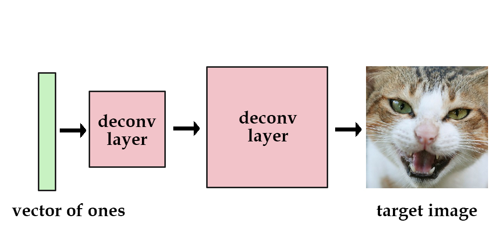
Let's say we had a network comprised of a few deconvolution layers. We set the input to always be a vector of ones. Then, we can train the network to reduce the mean squared error between itself and one target image. The "data" for that image is now contained within the network's parameters.
Now, let's try it on multiple images. Instead of a vector of ones, we'll use a one-hot vector for the input. [1, 0, 0, 0] could mean a cat image, while [0, 1, 0, 0] could mean a dog. This works, but we can only store up to 4 images. Using a longer vector means adding in more and more parameters so the network can memorize the different images.
To fix this, we use a vector of real numbers instead of a one-hot vector. We can think of this as a code for an image, which is where the terms encode/decode come from. For example, [3.3, 4.5, 2.1, 9.8] could represent the cat image, while [3.4, 2.1, 6.7, 4.2] could represent the dog. This initial vector is known as our latent variables.
Choosing the latent variables randomly, like I did above, is obviously a bad idea. In an autoencoder, we add in another component that takes in the original images and encodes them into vectors for us. The deconvolutional layers then "decode" the vectors back to the original images.
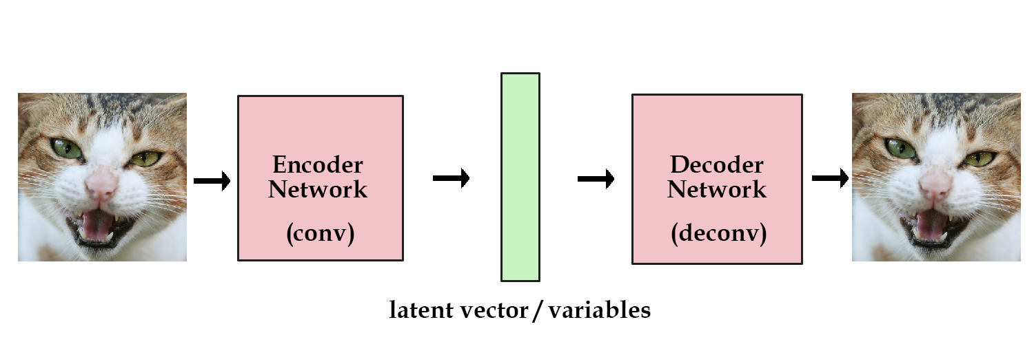
We've finally reached a stage where our model has some hint of a practical use. We can train our network on as many images as we want. If we save the encoded vector of an image, we can reconstruct it later by passing it into the decoder portion. What we have is the standard autoencoder.
However, we're trying to build a generative model here, not just a fuzzy data structure that can "memorize" images. We can't generate anything yet, since we don't know how to create latent vectors other than encoding them from images.
There's a simple solution here. We add a constraint on the encoding network, that forces it to generate latent vectors that roughly follow a unit gaussian distribution. It is this constraint that separates a variational autoencoder from a standard one.
Generating new images is now easy: all we need to do is sample a latent vector from the unit gaussian and pass it into the decoder.
In practice, there's a tradeoff between how accurate our network can be and how close its latent variables can match the unit gaussian distribution.
We let the network decide this itself. For our loss term, we sum up two separate losses: the generative loss, which is a mean squared error that measures how accurately the network reconstructed the images, and a latent loss, which is the KL divergence that measures how closely the latent variables match a unit gaussian.
generation_loss = mean(square(generated_image - real_image))
latent_loss = KL-Divergence(latent_variable, unit_gaussian)
loss = generation_loss + latent_loss
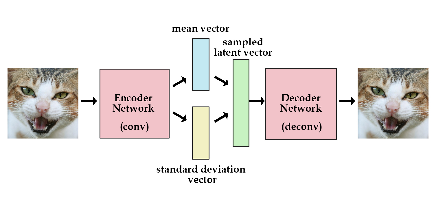
In order to optimize the KL divergence, we need to apply a simple reparameterization trick: instead of the encoder generating a vector of real values, it will generate a vector of means and a vector of standard deviations.
This lets us calculate KL divergence as follows:
# z_mean and z_stddev are two vectors generated by encoder network
latent_loss = 0.5 * tf.reduce_sum(tf.square(z_mean) + tf.square(z_stddev) - tf.log(tf.square(z_stddev)) - 1,1)
When we're calculating loss for the decoder network, we can just sample from the standard deviations and add the mean, and use that as our latent vector:
samples = tf.random_normal([batchsize,n_z],0,1,dtype=tf.float32)
sampled_z = z_mean + (z_stddev * samples)
In addition to allowing us to generate random latent variables, this constraint also improves the generalization of our network.
To visualize this, we can think of the latent variable as a transfer of data.
Let's say you were given a bunch of pairs of real numbers between [0, 10], along with a name. For example, 5.43 means apple, and 5.44 means banana. When someone gives you the number 5.43, you know for sure they are talking about an apple. We can essentially encode infinite information this way, since there's no limit on how many different real numbers we can have between [0, 10].
However, what if there was a gaussian noise of one added every time someone tried to tell you a number? Now when you receive the number 5.43, the original number could have been anywhere around [4.4 ~ 6.4], so the other person could just as well have meant banana (5.44).
The greater standard deviation on the noise added, the less information we can pass using that one variable.
Now we can apply this same logic to the latent variable passed between the encoder and decoder. The more efficiently we can encode the original image, the higher we can raise the standard deviation on our gaussian until it reaches one.
This constraint forces the encoder to be very efficient, creating information-rich latent variables. This improves generalization, so latent variables that we either randomly generated, or we got from encoding non-training images, will produce a nicer result when decoded.
How well does it work?
I ran a few tests to see how well a variational autoencoder would work on the MNIST handwriting dataset.
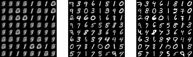
left: 1st epoch, middle: 9th epoch, right: original
Looking good! After only 15 minutes on my laptop w/o a GPU, it's producing some nice results on MNIST.
Here's something convenient about VAEs. Since they follow an encoding-decoding scheme, we can compare generated images directly to the originals, which is not possible when using a GAN.
A downside to the VAE is that it uses direct mean squared error instead of an adversarial network, so the network tends to produce more blurry images.
There's been some work looking into combining the VAE and the GAN: Using the same encoder-decoder setup, but using an adversarial network as a metric for training the decoder. Check out this paper or this blog post for more on that.
You can get the code for this post on my Github. It's a cleaned up version of the code from this post.