It's been shown many times that convolutional neural nets are very good at recognizing patterns in order to classify images. But what patterns are they actually looking for?
I attempted to recreate the techniques described in Visualizing and Understanding Convolutional Networks to project features in the convnet back to pixel space.
In order to do this, we first need to define and train a convolutional network. Due to lack of training power, I couldn't train on ImageNet and had to use CIFAR-10, a dataset of 32x32 images in 10 classes. The network structure was pretty standard: two convolutional layers, each with 2x2 max pooling and a reLu gate, followed by a fully-connected layer and a softmax classifier.
We're only trying to visualize the features in the convolutional layers, so we can effectively ignore the fully-connected and softmax layers.
Features in a convolutional network are simply numbers that represent how present a certain pattern is. The intuition behind displaying these features is pretty simple: we input one image, and retrieve the matrix of features. We set every feature to 0 except one, and pass it backwards through the network until reaching the pixel layer. The challenge here lies in how to effectively pass data backwards through a convolutional network.
We can approach this problem step-by-step. There are three main portions to a convolutional layer. The actual convolution, some max-pooling, and a nonlinearity (in our case, a rectified linear unit). If we can figure out how to calculate the inputs to these units given their outputs, we can pass any feature back to the pixel input.
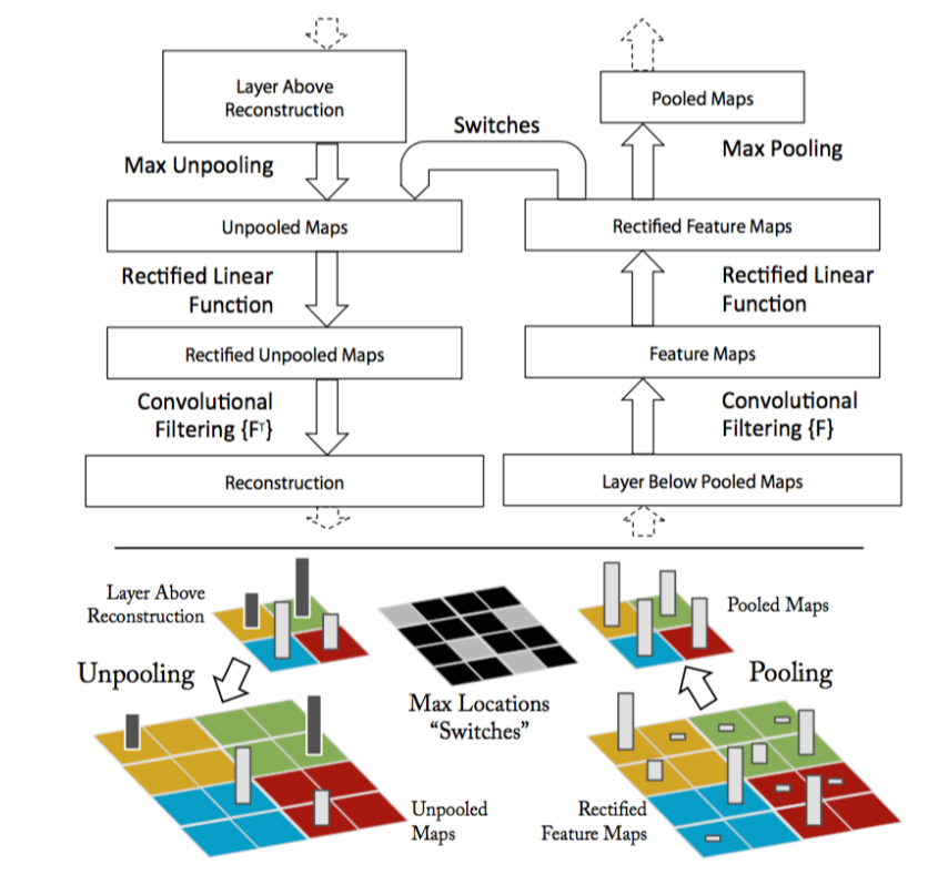
image from Visualizing and Understanding Convolutional Networks
Here, the paper introduces a structure called a deconvolutional layer. However, in practice, this is simply a regular convolutional layer with its filters transposed. By applying these transposed filters to the output of a convolutional layer, the input can be retrieved.
A max-pool gate cannot be reversed on its own, as data about the non-maximum features is lost. The paper describes a method in which the positions of each maximum is recorded and saved during forward propagation, and when features are passed backwards, they are placed where the maximums had originated from. In my recreation, I took an even simpler route and just set the whole 2x2 square equal to the maximum activation.
Finally, the rectified linear unit. It's the easiest one to reverse, we just need to pass the data through a reLu again when moving backwards.
To test these techniques out, I trained a standard convolutional network on CIFAR-10. First, I passed one of the training images, a dog, through the network and recorded the various features.
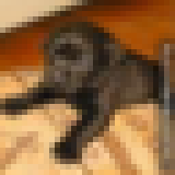
our favorite dog
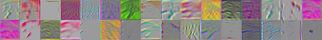
first convolutional layer (features 1-32)
As you can see, there are quite a variety of patterns the network is looking for. You can see evidence of the original dog picture in these feature activations, most prominently the arms.
Now, let's see how these features change when different images are passed through.
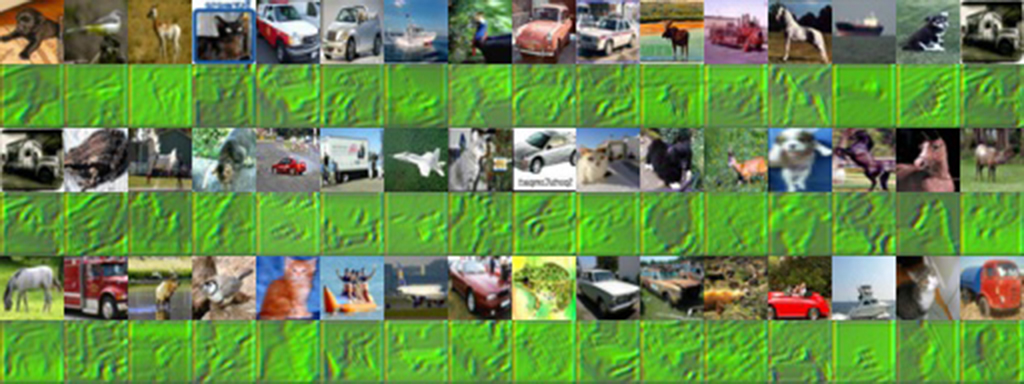
first convolutional layer (feature #7)
This image shows all the different pixel representations of the activations of feature #7, when a variety of images are used. It's clear that this feature activates when green is present. You can really see the original picture in this feature, since it probably just captures the overall color green rather than some specific pattern.
Finally, to gain some intuition of how images activated each feature, I passed in a whole batch of images and saved the maximum activations.
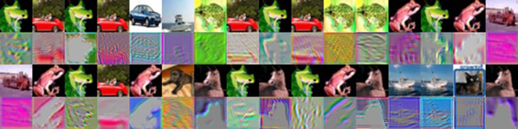
maximum activations for 32 features
Which features were activated by which images? There's some interesting stuff going on here. Some of the features are activated simply by the presence of a certain color. The green frog and red car probably contained the most of their respective colors in the batch of images.
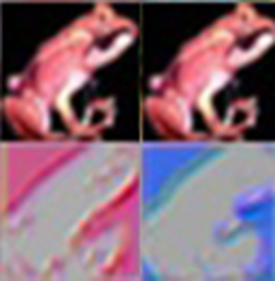
two activations from the above image
However, here are two features which are activated the most by a red frog image. The feature activations show an outline, but one is in red and the other is in blue. Most likely, this feature isn't getting activated by the frog itself, but by the black background. Visualizing the features of a convolutional network allows us to see such details.
So, what happens if we go farther, and look at the second convolutional layer?
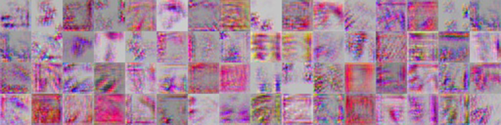
second convolutional layer (64 features)
I took the feature activations for the dog again, this time on the second convolutional layer. Already some differences can be spotted. The presence of the original image here is much harder to see.
It's a good sign that all the features are activated in different places. Ideally, we want features to have minimal correlation with one another.
Finally, let's examine how a second layer feature activates when various images are passed in.
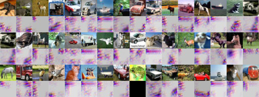
second convolutional layer (feature #9)
For the majority of these images, feature #9 activated at dark locations of the original image. However, there are still outliers to this, so there is probably more to this feature than that.
For most features, it's a lot harder to tell what part of the image activated it, since second layer features are made of any linear combination of first layer features. I'm sure that if the network was trained on a higher resolution image set, these features would become more apparent.
The code for reproducing these results are available on my Github