A Brief Examination of Generative Models

Let's explore some generative models. There's a nice variety of them around. How well can the various methods model a given dataset? What are their flaws and strengths?

I'm interested in how well generative models handle mode coverage. Let's say my dataset has images of five cat breeds. How is each breed reflected in the generated images? If one breed is less prominent in the data, does that affect the accuracy of its generated versions?

The goal with this project was to get a deeper sense of how each generative model method works, and in what unique ways they can fail. We will take a look at 1) variational auto-encoders, 2) generative adversarial networks, 3) auto-regressive samplers, and 4) diffusion models.

Code for all these experiments is available at https://github.com/kvfrans/generative-model.

The Dataset

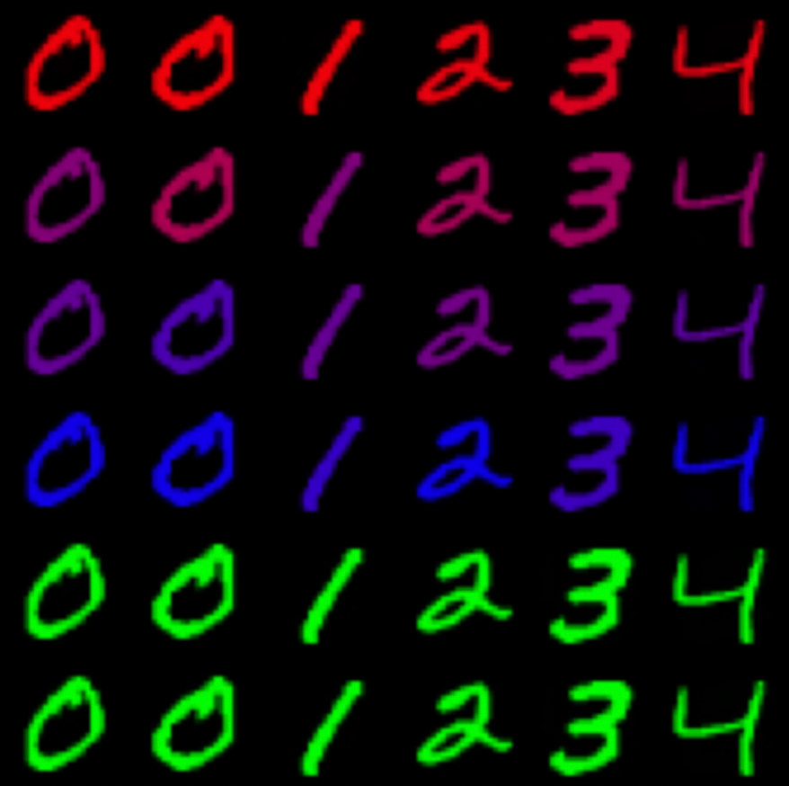
To get a cleaner look at the various models, I opted to create an artificial dataset rather than use natural images. The dataset is based off of MNIST digits. But, I've put some tricks in how the dataset is constructed. We'll use only these five digits, which I will refer to as "0A, 0B, 1, 2, 3, 4".

The main twist is that each digit is present in the dataset at differing frequencies. ["0A, 0B, 1, 2"] are included at the same equal frequency. "3" is half as likely to be sampled, and "4" is a quarter as likely. So, the digits "3" and "4" are less present than the other digits. A strong generative model should be able to correctly model these frequency differences.

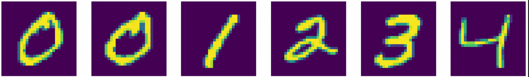
You'll notice that 0 is in the list twice. This is intentional. There are two kinds of zeros, but they are quite similar. I'm curious if the models can correctly generate both kinds of digits.

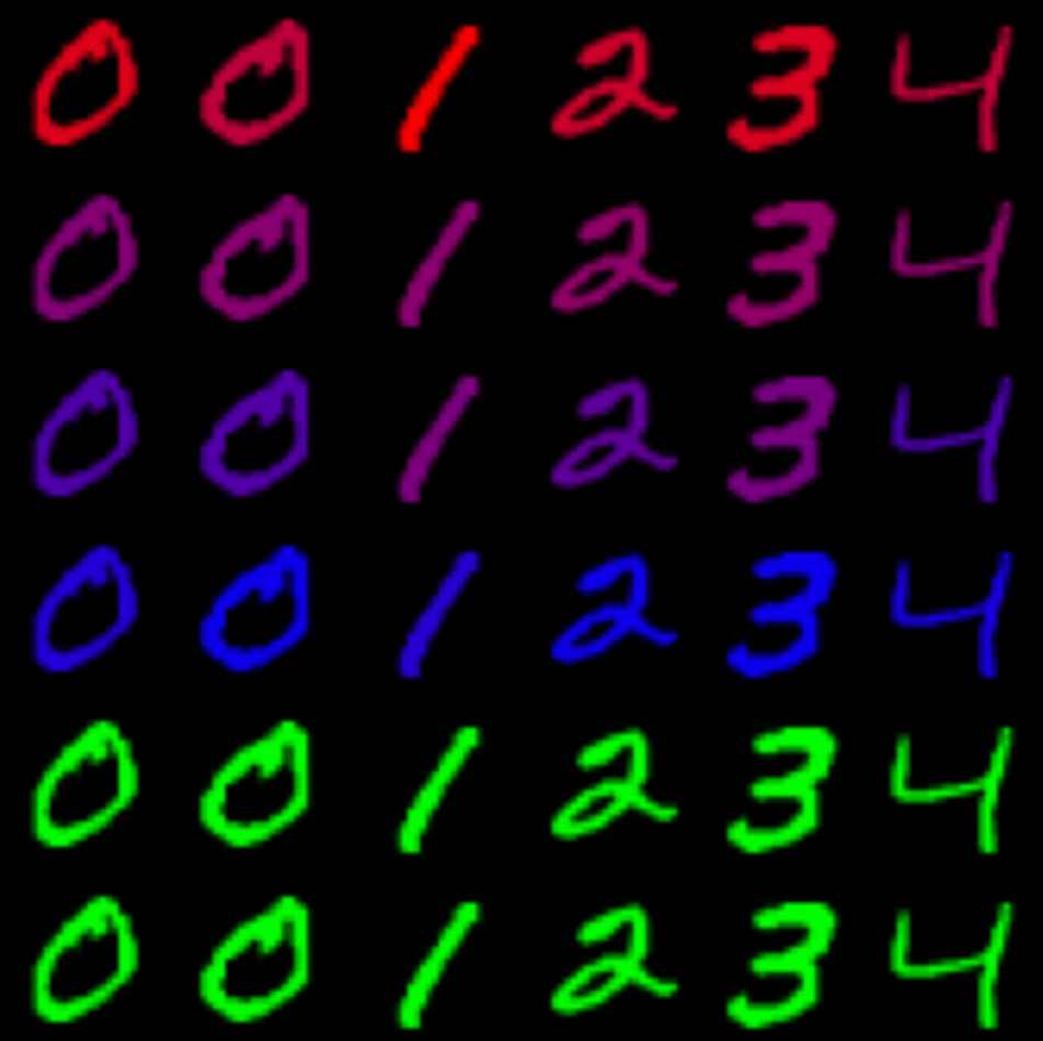
We'll also add a second dimension of variation -- color. Again, we're going to put some twists on the frequencies here so everything isn't just uniform. Each digit has a (1/3) chance to be pure green. With (2/3) chance, the digit will instead be a random linear interpolation between red and blue. In other words, there is a continuous distribution of colors between red and blue, and a discontinuous set of pure green digits.

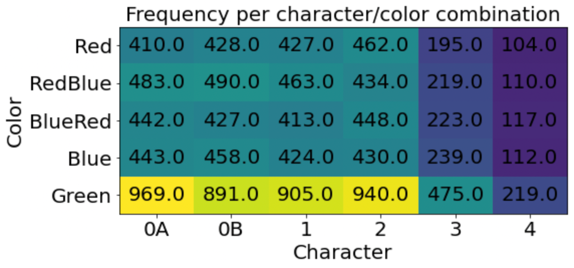
How will we measure mode coverage? First, we will need a way to categorize generated digits into one of the 30 possible bins. Let's train a classifier network.

Actually, that's a trap and we won't. There's a much simpler way to classify them; nearest neighbors. To classify a digit, we'll simply loop over the six possible MNIST digits and find the one with the lowest error. We'll do the same for the average color. In this way, we can cheaply categorize digits to look at frequencies.

Accuracy is straightforward as well. Once a digit has been categorized, measure the distance between the generated digit and its closest match. That will be the accuracy.

Oracle Network

As a starting point, let's construct a network that can access privileged information. We'll call it the oracle network. This network will take as input a vector containing a one-hot encoding of the MNIST digit, and a three-vector of colors. Given this input, it must recreate the matching colored digit.

The oracle network has a straightforward learning objective. It only has to memorize colored versions of the six digits, and doesn't need to model any sort of probability distribution. We can train the network with a mean-squared error loss.

I'm using JAX to write the code for these experiments. The network structure is a few fully-connected linear layers, interspersed with tanh activations.

activation = nn.tanh
class GeneratorLinear(nn.Module):
    @nn.compact
    def __call__(self, x):
        # Input: N-length vector.
        x = nn.Dense(features=64)(x)
        x = activation(x)
        x = nn.Dense(features=128)(x)
        x = activation(x)
        x = nn.Dense(features=28*28*3)(x)
        x = nn.sigmoid(x)
        # Output: 28x28x3 image.
        x = x.reshape(x.shape[0], 28, 28, 3)
        return x

Throughout this project, we'll do our best to use this same network structure for all the methods.

As expected, it's an easy task. Memorizing these MNIST digits is simple. Trickier will be generating them at the right frequencies.

Variational Auto-Encoder

The first generative modelling method we'll examine is the variational auto-encoder (VAE).

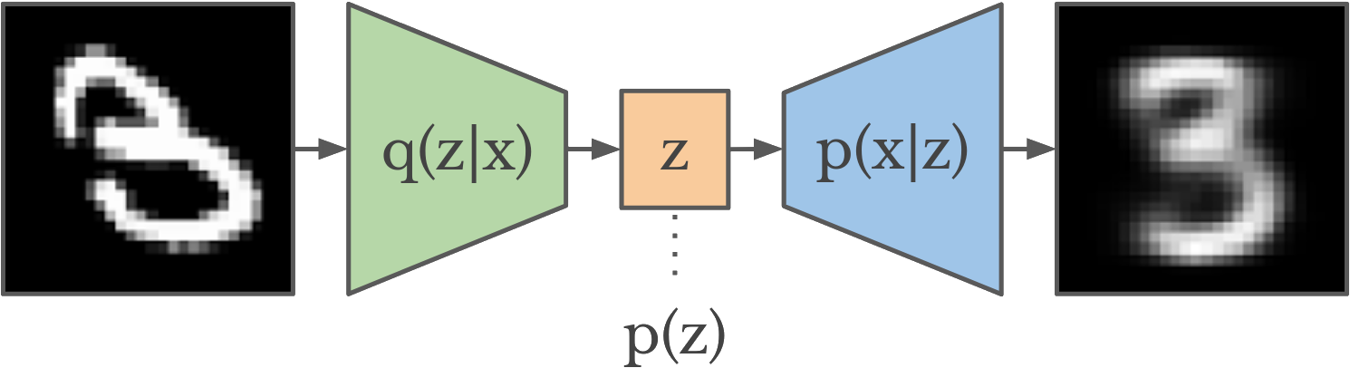
The VAE works by jointly training an encoder and decoder network. The encoder takes in an image as input, and compresses it down to an N-length latent vector $z$. This latent vector is then given to the decoder, which recreates the original image.

The catch is that we're not happy just encoding and decoding an existing image. We want to generate images, which means sampling them from a random distribution. What is the distribution? It's $P(z)$. Unfortunately $P(z)$ is high dimensional and intractable to sample from.

Instead, we shape $P(z)$ so it's in a form that we can work with. We'll have the encoder output not a latent vector, but a Gaussian parametrized by mean and log-variance. We also apply a KL divergence objective between the output and the unit Gaussian ($\mu = 0; \sigma = 1$). This objective encourages the model so that $P(z)$ looks similar to the unit Gaussian.

This shaping means we can approximate $P(z)$ by sampling $z$ from the unit Gaussian. And that's precisely what we do to generate new images -- sample a random latent variable, then pass it through the decoder.

For more on VAEs, check out this post and this newer one.

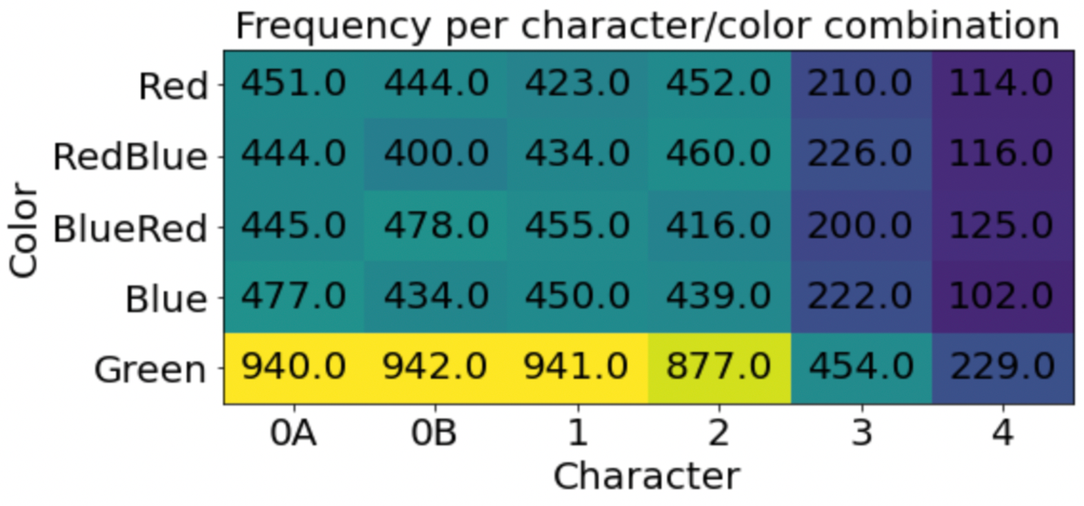
The VAE is quite stable to train, and it does a good job. It's surprising how well the frequencies match the ground truth. The errors are greater for digits that are less frequently seen during training. Soon we'll see that a well-behaved objective is not to be taken for granted.

Generative Adversarial Networks

Next up is the generative adversarial network (GAN). GANs attack the problem that measuring reconstruction via a mean-squared error loss is not ideal. Such a loss often results in a blurry image -- colors will collapse to the mean, so a digit that is either red or blue will be optimized to be purple. In the GAN setup, reconstruction error is instead measured by a learned discriminator network.

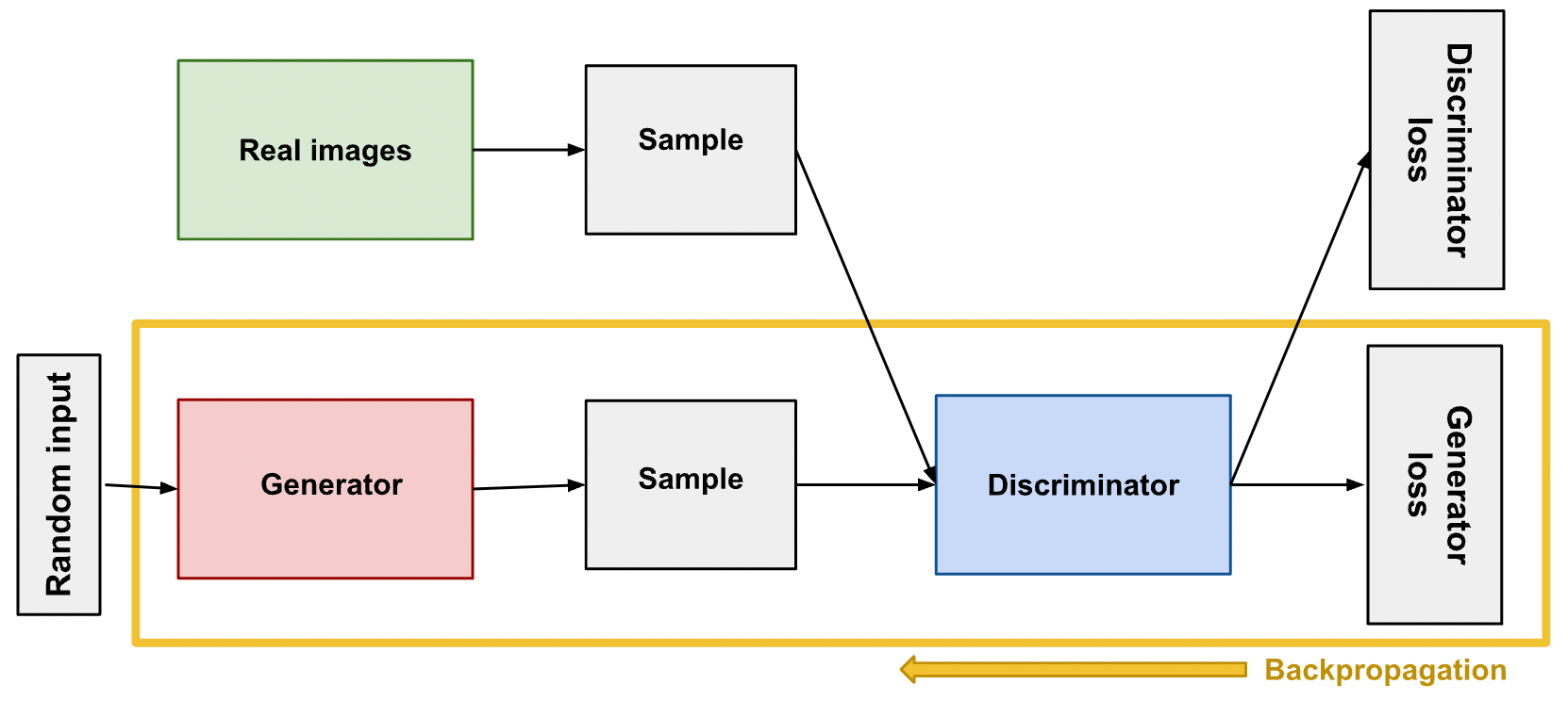
The setup is as follows. The generator takes random noise as input, and produces fake images. The images are then passed to the discriminator, which predicts whether the image is real or fake. The generator's objective is to maximize the probability that the discriminator classifies its images as real.

Meanwhile, the discriminator is trained on both real and fake images, and is optimized to classify them accordingly. Thus, there is an adversarial game here. At the Nash equilibrium, the generator is producing images that exactly match the distribution of real images.

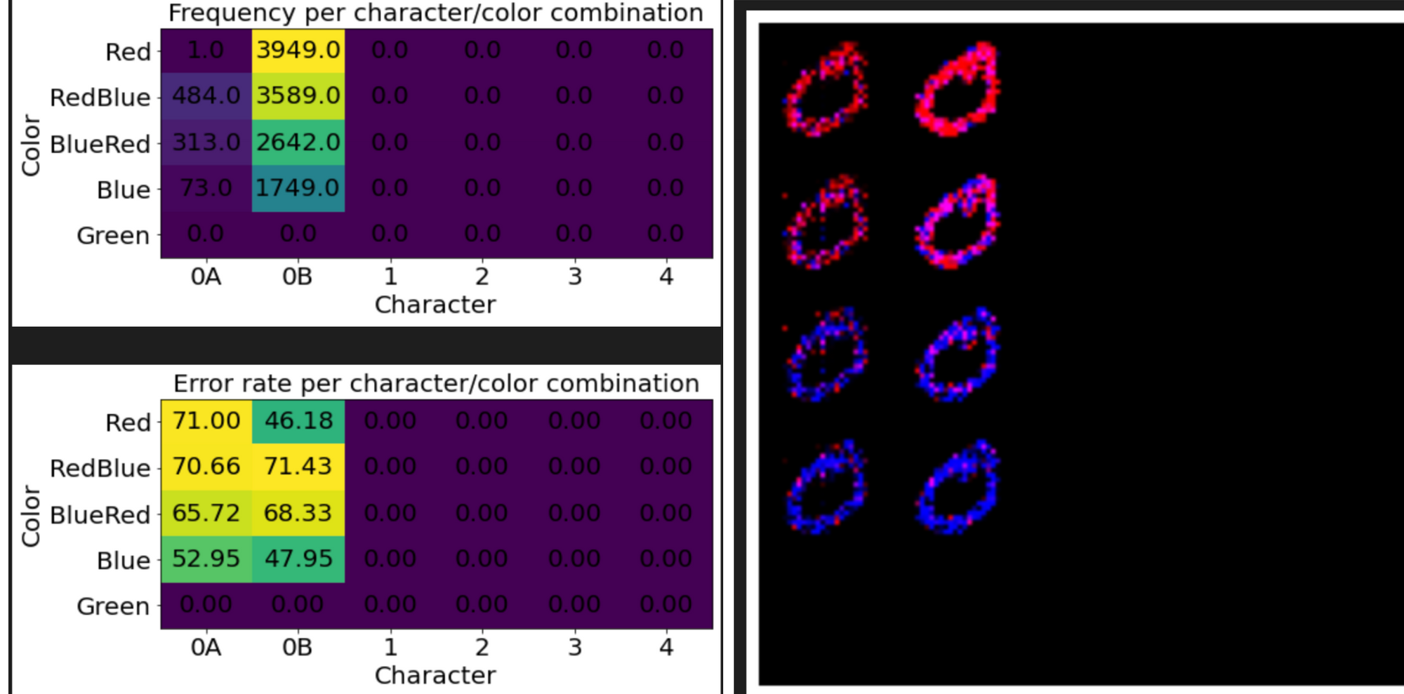
Looking at the frequencies gives a hint to a key flaw in GANs. They often suffer from "mode collapse", where the generator fails to capture the entire spectrum of data, and instead produces a limited subset. In the results above, we see a generator that produces only 2s, and a separate trial that produces only 0s.

The mode collapse issues arises because the discriminator assesses each image independently. Thus there is no picture of the distribution of generated images, which is needed to assess diversity. In theory, mode collapse is solved in the optimal equilibrium -- if a generator is producing only 0s, the discriminator can penalize 0s, forcing the generator to produce something else, and so on. In practice, it is hard to escape this local minima.

One way to address mode collapse is via minibatch discrimination. In this idea, the discriminator receives privileged information about the batch as a whole. For each image, the discriminator can see the average distance of the image to the rest of the batch, in a learned feature space. This setup allows the discriminator to learn what statistics should look like in a batch of real images, thus forcing the generator to match those statistics.

Does it work? Well, we are doing better on the frequencies. But the quality of the results have taken a hit. GANs are quite unstable to train due to their adversarial nature. The discriminator must provide a clean signal for the generator to learn from, and often times this signal will be lost or diminished.

Auto-Regressive Sampling

In this next section, we'll take a look at a method that explicitly models the image probability distribution $P(x)$.

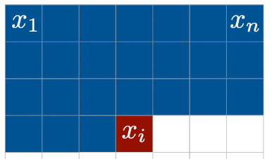
The issue with modelling $P(x)$ directly is that the image space is high-dimensional. Instead, we need to break it into smaller components. PixelRNN breaks down an image into a sequence of pixels. If we can model $P(x_t|x_0...x_{t-1})$, then $P(x)$ becomes the product of these individual probabilities. In other words -- generate an image pixel-by-pixel.

To model the probability distribution of a pixel, it helps to break the color into a set of discrete bins. I chose to represent each RGB channel as 8 possible options. Together this results in $8^3 = 512$ bins for each pixel. Our model will be a neural network that outputs a probability distribution over these 512 bins, given the preceding pixels.

To process our image, we'll flatten each image into a $28*28 = 784$-length vector. The vector has 3 channels for the color, and an additional 2 channels for the normalized XY position of that pixel. 2 more channels are set to $(1-XY)$ coordinates. It's also helpful to include a boolean channel that is 1 if the pixel is on the right-most X boundary -- this information helps in modelling the jump between rows of an image.

In the original PixelRNN setup, the neural network model is a recurrent network. It ingests a sequence of pixels recurrently, updating its hidden state, then using the final hidden state to predict the next pixel. I tried this setup but I had quite a hard time getting the model to converge.

Instead, we're going to use a hacky flattened version. The model gets to see the past 64 pixels, each which has 8 channels, for a total of $512$ channels per input. That's not bad at all. A flattened network is often inefficient because there is redundancy in treating each channel as separate, when in reality there is some temporal structure to it. But in our case, it's easier to learn a flattened feedforward network than a recurrent one due to stability in training.

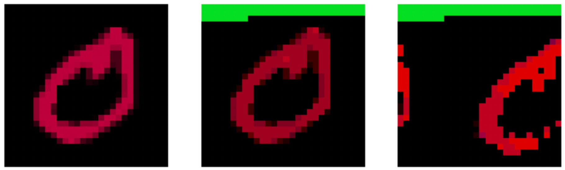
During implementation, I ran into some troubles. It was easy to mess up the sampling procedure. The network needs to iterate through the image, predicting the next pixel and placing that pixel in the correct space. You can see in this example that the rows don't match up correctly so the digit is shifted.

Even with the correct sampling, the network's results aren't great.

A key issue with auto-regressive sampling is that it's easy to leave the training distribution. Since we're generating each image a pixel at a time, if any of those pixels gets generated wrong, then the subsequent pixels will likely also be wrong. So the model needs to generate many pixels without any errors -- a chance that quickly decays to 0 as the sequence length increases.

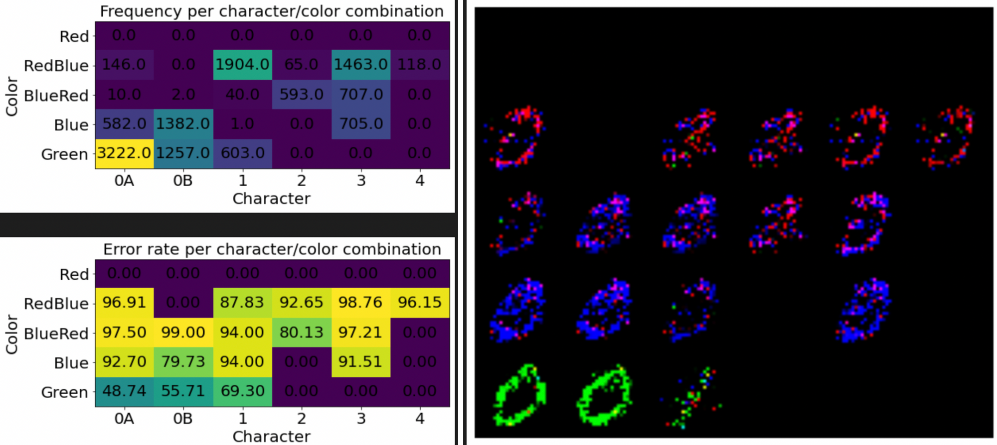
We can see in the example images that the generated digits start to lose structure. The images all sort of resemble MNIST digits, but they don't have a coherent shape.

The frequencies of the generated digits are also quite wrong. This issue points to another flaw in auto-regressive sampling. P(x) is split into a sequence of probabilities, and important decisions have to be made early on. As an example, the choice for what digit to generate might occur in the 28th pixel, because that pixel is blank for a 2 or 3. It's not great for stability to have big sways in probabilities during certain pixel locations.

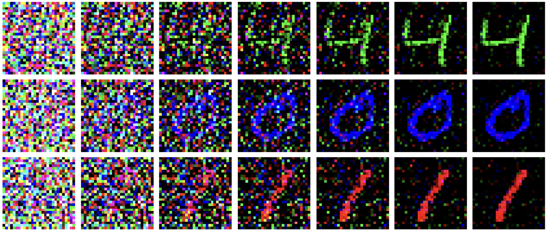
Diffusion Models

Our final generative modelling method also samples auto-regressively, but does so over time instead of over pixels.

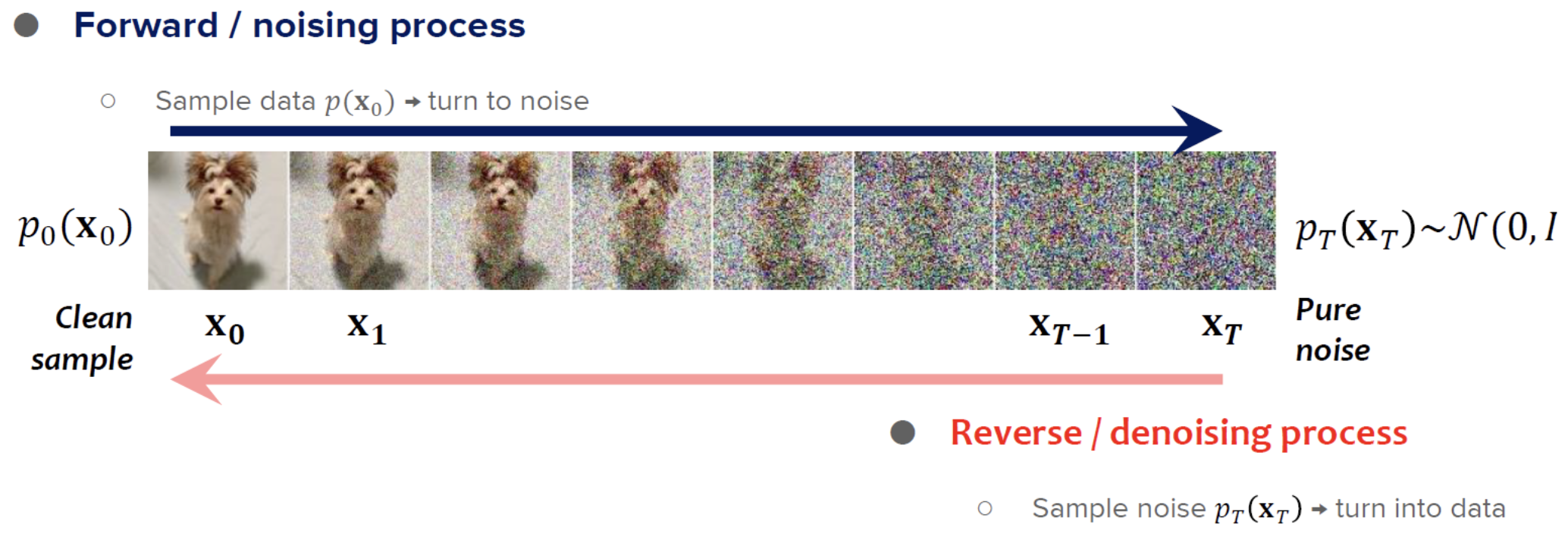
We'll start by defining a noising process. This process will take an image from the dataset, and progressively add Gaussian noise to it. By the end of the process (say, 300 timesteps), the image is purely Gaussian noise.

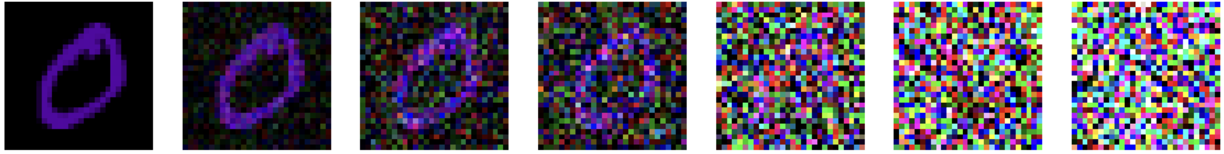
The task for the diffusion model is now to reverse that process. Starting from a pure Gaussian image, it should iteratively remove the noise until the original image is recreated. The nice property about recreating an image sequentially is that decisions can be spread out. The first few denoising steps might define the outline of an image, while later steps add in the details.

Gaussian noise gives us a few nice properties.

• Applying two steps of Gaussian noise to an image is equivalent to applying one step with greater variance. This property lets us easily simulate an image with $T$ steps of noising, in a single operation.

• If the forward process $p(x_{t+1}| x_{t})$ is Gaussian, then the reverse process $q(x_{t}| x_{t+1})$ is also Gaussian given the variance is low. (https://lilianweng.github.io/posts/2021-07-11-diffusion-models/)

Because of the second property, we can approximate the reverse process as a Gaussian. The variances are fixed, but we need to learn the mean of that distribution -- that's what our network does.

In the original DDPM paper, the network predicts the noise that was added, not the original image. I found that this was hard to achieve. Because our model is quite small, it's hard to compress 28*28*3 samples of independent noise into a feedforward bottleneck. In contrast, it's simpler to compress the original image since there are only a few MNIST digits. The noise can be recovered via noise = noisy_image - predicted_original_image.

Note that the denoising process is a Gaussian at every timestep. So while we're predicting the mean with our learned network, we also add back noise. The variance of this noise follows the pre-determined schedule so it decreases over time.

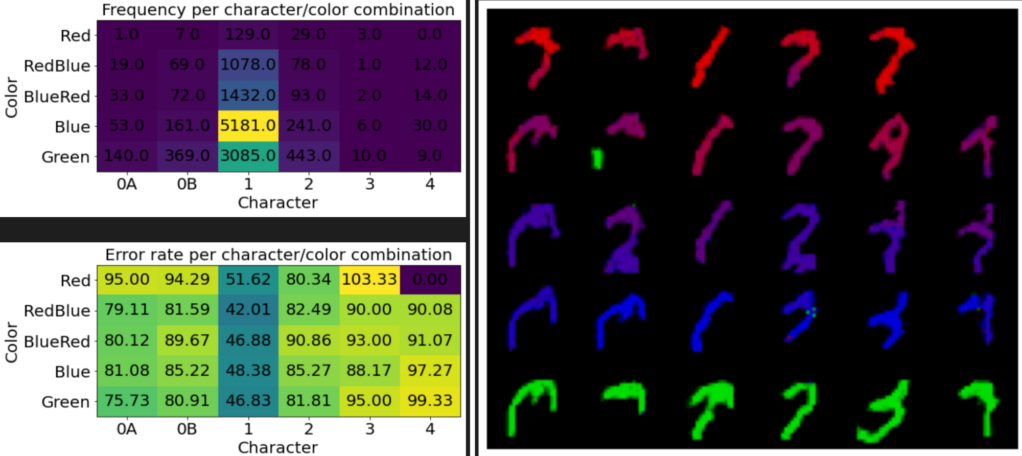
What do the metrics show?

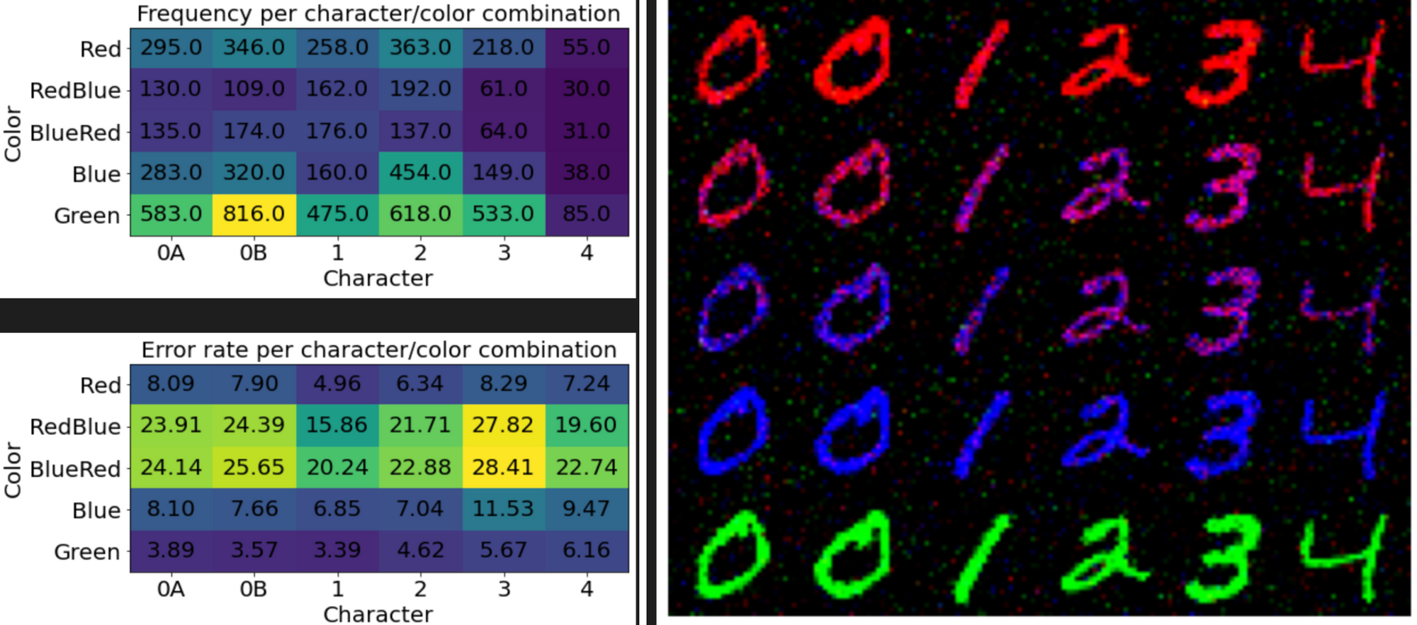
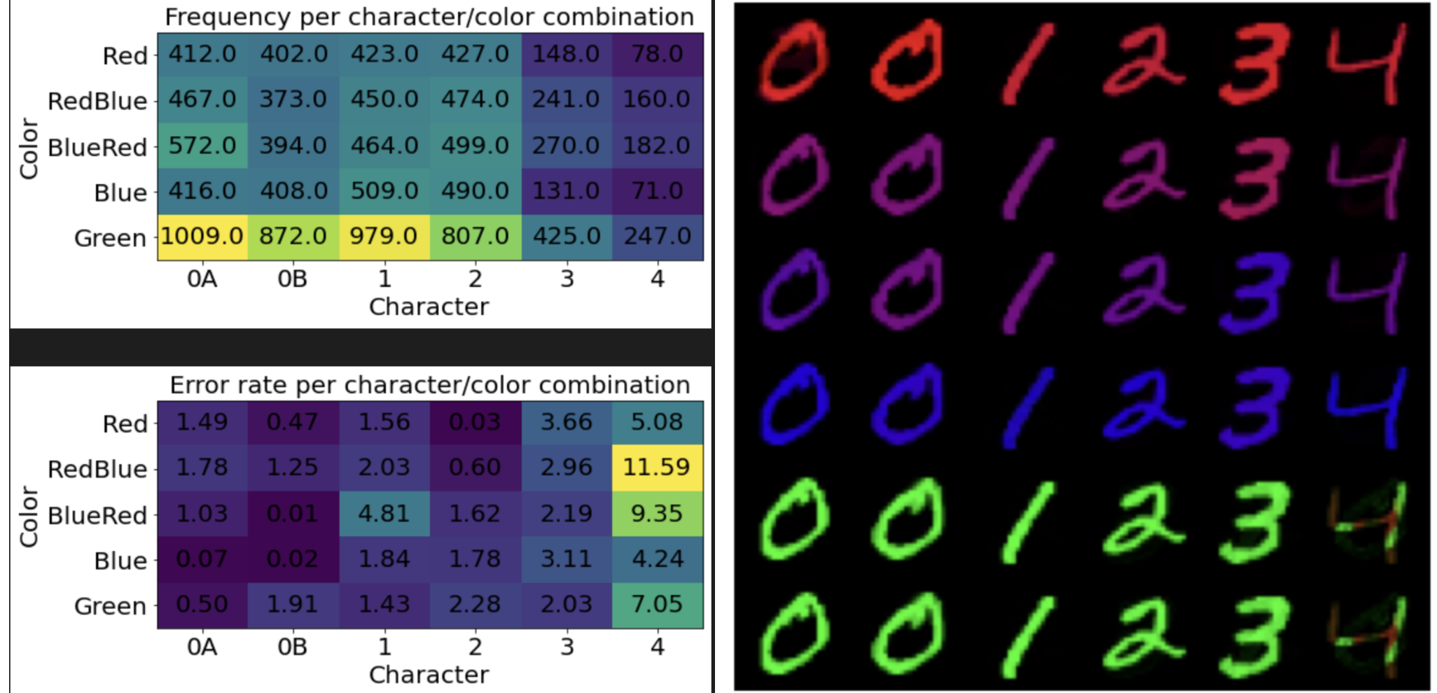
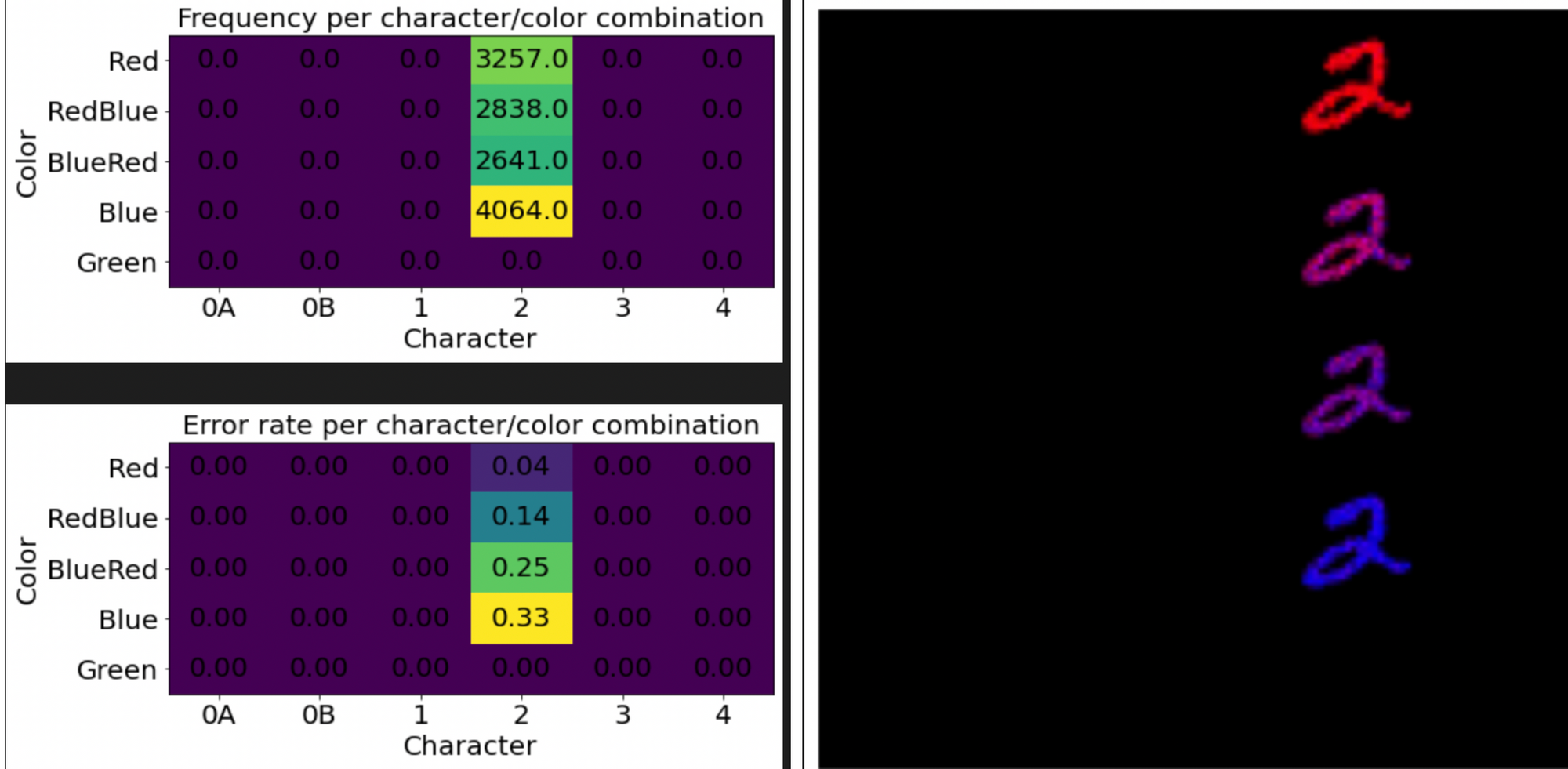
Works nicely. The frequencies aren't as well-matched as the VAE, but it's at least covering all the modes. That's better than the GAN or PixelRNN.

The error rates are interesting. The highest error isn't by shape, but by color. Examining the generated images, it looks like the model has trouble deciding if it wants to make the digits red or blue. Really, those pixels should all be a shade of purple, with all pixels being the same shade.

As always, code for everything here is available at https://github.com/kvfrans/generative-model.