In my last post I described the DRAW model of recurrent auto-encoders. As far as I've seen, the only implementations of DRAW floating around Github deal with the MNIST dataset. While they are helpful for reference, I wanted to have a model that could successfully generate photographs, not just black-and-white digits.
In this post, I'll go over the steps and thinking behind taking a working implementation of DRAW, and adjusting it to work on colored pictures.
The first question to ask is: what changed? In the original DRAW model, the input data consists of many 28x28 arrays of either 1 or 0. There's already a problem: images don't consist of only pure white or pure black pixels. They have a range, usually from 0 - 255.
The loss function
To account for this, we'll replace the log likelihood loss function with an L2 loss, which takes a sum of the squared difference between each pixel.
//log likelihood loss func
self.generation_loss = tf.reduce_mean(-tf.reduce_sum(self.images * tf.log(1e-10 + self.generated_images) + (1-self.images) * tf.log(1e-10 + 1 - self.generated_images),1))
//l2 loss func
self.generation_loss = tf.nn.l2_loss(x - self.generated_images)
Although these two functions compute loss differently, they're essentially accomplishing the same task: a measurement of how well our image matches the original.
On a side note, this also brings up a key part in the variational autoencoder: balance between latent and generation loss.
The lower our latent loss is, the closer our latent vector distribution is to a unit gaussian, which forces the model to generalize. However, we also want the generation loss to be low, and have accurate reconstructions.
In some implementations, such as this one by ikostrikov, the total loss is the sum of the latent and generation loss. By changing the generation loss to L2, the "correct" ratio may not be one to one anymore.
I didn't look any farther into using training/test splits to find a perfect ratio, although that may be worth trying in the future. For our current model, a one-to-one ratio between L2 generation loss and the KL latent loss performed well.
Color channels and attention
In the DRAW model, we calculate an attention patch for every timestep, dictating where the model is observing.
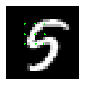
green dots mark attention location
To allow for colored images, we need to decide how to handle attention with multiple color channels. When a human looks at something, it's looking at the same area for all colors. Therefore, the attention location should be exactly the same for all color channels in our model.
How can this be done in practice? It turns out we don't need to mess with any of the code for the attention filter.
Instead, we treat each color channel (red, green, blue) as a separate image. We're already handling multiple images simultaneously in our minibatch, so it all fits together nicely.
Essentially, instead of having a batchsize of 64, we have a "batchsize" of 64*3. The only thing we need to do now is take our 64-length vector of attention parameters and stretch it out into a 64*3 vector, with every three values being the same.
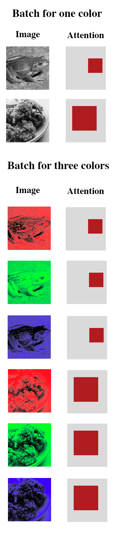
structure of stretched out batch, from a batch size of two images
Once we've passed the color-separated through the attention gate, we then have a 5x5 matrix for each color channel. These can be concatenated to form a 5x5x3 matrix for each image. Finally, we pass this 5x5x3 into the encoder, instead of the 5x5 in single-color DRAW.
Results
How did it do? I ran the model trained on the celebA dataset, resized down to 64x64 each image.
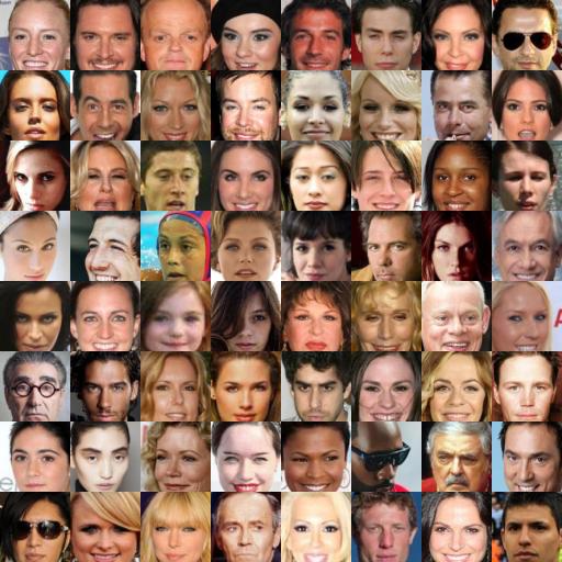
the original images
the recreated images
The results are pretty blurry. However, they do resemble faces and match up to their respective original images.
The interesting part is how attention is shifted to accommodate a dataset of faces. We can plot the attention parameters for each face at every timestep to visualize it.
attention patches at each timestep
attention patches on top of image
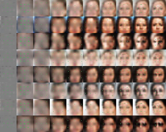
non-animated version
These dots help us see where the network is assigning its attention at any given timestep.
We can see how at step 3, the attention starts out spread out and fills in the edges of the images. As the timesteps go on, the attention patch shrinks, with the smallest at the final timestep.
This makes sense when looking at how the images are created, starting from the out and working its way inwards with increasing detail.
An interesting thing to note it that these attention patches are in relatively the same location, regardless of the face being created. The DRAW video has attention move differently when different digits are being recreated.
How can it be improved?
The results show that the model works, but the results are quite blurry. There are some potential steps we can take to make them better.
Train Longer: I only trained the model for one epoch (~2400 iterations). That's a pretty low amout of training given the data size, and more training is probably the next best step.
Bigger latent variable: Currently, the latent variable is a vector of 10 real numbers. If we increase this, more information, and therefore more details about the image, can be passed. This has the downside that the model might overfit the current dataset, so we need a balance.
More timesteps: If we give the model more timesteps, it will have more operations in which to update the image, ideally allowing it to create more detail. In addition, the way DRAW is setup has an additional latent variable for every timestep, so more information is passed as well (whether this is good or bad is up for debate).
Better loss function: In our color DRAW model, we're using an L2 pixel-by-pixel loss. The problem here is the model may get stuck in the middle of two possibilities. For example, if a certain pixel could either be bright red or completely black, the model would converge to the average of a dark red, which is neither of the options. This is why it's often better to be using classification rather than regression, as an average may often be incorrect.
The paper Autoencoding beyond pixels using a learned similarity metric describes a combination of a generative adversial network and a variational autoencoder.
In short, a generative adversial network naturally trains a discriminator network which attempts to tell real and fake images apart. It will take some tweaking, but we can use this discriminator as a measurement of how close we are to an original image, rather than an L2 loss.
Using the GAN usually leads to more crisp images, as we don't suffer from blurriness caused by converging to an average as described above. The downsides are that we introduce more parameters to train, and the GAN has a chance to become unstable and diverge.
As usual, the code for this project can be found on my Github.