A few weeks ago I made a post on variational autoencoders, and how they can be applied to image generation. In this post, we'll be taking a look at DRAW: a model based off of the VAE that generates images using a sequence of modifications rather than all at once.
In most image generation methods, the actual generation network is a bunch of deconvolution layers. These map from some initial latent matrix of parameters to a bigger matrix, which then maps to an even bigger matrix, and so on.

how images are generated from deconvolutional layers. [source]
However, there's another way to think about image generation. In the real world, artists don't create paintings instantly. It's a sequence of brush strokes that eventually make up something that looks amazing.
DRAW attempt to replicate this behavior. Instead of creating an image instantly, it uses a recurrent neural network as both the encoder and decoder portions of a typical variational autoencoder. Every timestep, a new latent code is passed from the encoder to the decoder.
simple recurrent VAE setup
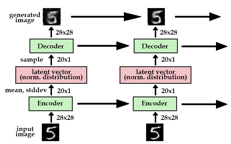
Here's a model of a simplified version of DRAW. If you saw the diagram in my previous VAE post, you would notice that the first column in the recurrent model is exactly the same as a typical variational autoencoder. The difference here is that instead of generating a final image directly, we break up its generation into many iterations. Every iteration, the model improves upon its generated image until the final image (hopefully) looks like the original.
Above, the horizontal arrows represent recurrent neural networks. These are fully-connected layers that maintain an internal hidden state along with taking in an input. In practice, we use LSTMs. The uppermost horizontal arrow simply represents the iterative construction of our goal image, as each timestep's image is simply elementwise addition.
new image = [the last image](shape=28x28) + [some improvements](shape=28x28)
By itself, this simple recurrent version of a variational autoencoder performs pretty well. We can successfully generate nice-looking MNIST images by iterative improvements.
MNIST results of recurrent VAE
However, artists in real life don't draw by continuously making small changes to the entire canvas. Brush strokes occur only in one portion of the image. In the cast of MNIST: when writing a 5, the typical person does not start from a blob and gradually erase portions until it looks nice. They just make one smooth motion following the shape of the 5.
The DRAW model acknowledges this by including an attention gate. This is the more complicated part of DRAW, so I'll start from a high-level explanation and go into detail on how attention is implemented.
An attention gate allows our encoder and decoder to focus on specific parts of our image.
Let's say we're trying to encode an image of the number 5. Every handwritten number is drawn a little differently: some portions may be thicker or longer than others. Without attention, the encoder would be forced to try and capture all these small nuances at the same time.
However, if the encoder could choose a small crop of the image every frame, it could examine each portion of the number one at a time.
> Reading MNIST [[video source]](https://www.youtube.com/watch?v=Zt-7MI9eKEo)The same goes for generating the number. The attention unit will determine where to draw the next portion of the 5, while the latent vector passed will determine if the decoder generates a thicker area or a thinner area.
> Writing MNIST [[video source]](https://www.youtube.com/watch?v=Zt-7MI9eKEo)In summary, if we think of the latent code in a VAE as a vector that represents the entire image, the latent codes in DRAW can be thought of as vectors that represent a brush stroke. Eventually, a sequence of these vectors creates a recreation of the original image.
But how does it work?
In the simple recurrent VAE model, the encoder takes in the entire input image at every timestep. Instead of doing this, we want to stick in an attention gate in between the two, so the encoder only receives the portion of our image that the network deems is important at that timestep. We will refer to this first attention gate as the "read" attention.
There's two parts to this attention gate: choosing the important portion, and cropping the image to get rid of the other parts.
We'll start with the first part. In order to determine which part of the image to focus on, we need some sort of observation to make a decision based on. In DRAW, we use the previous timestep's decoder hidden state. Using a simple fully-connected layer, we can map the hidden state to three parameters that represent our square crop: center x, center y, and the scale.
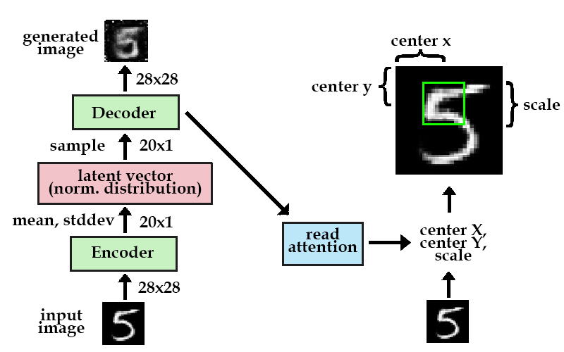
How the "read" attention gate works. Note the first timestep should have an attention gate but it is omitted for clarity. The attention gate shown is in the next timestep.
Now, instead of encoding the entire image, only a small of the image is encoded. This code is then passed through the system, and decoded back into a small patch.
We have a second attention gate after the decoder, that's job is to determine where to place this small patch. It's the same setup as the "read" attention gate, except the "write" attention gate uses the current decoder instead of the previous timestep's decoder.
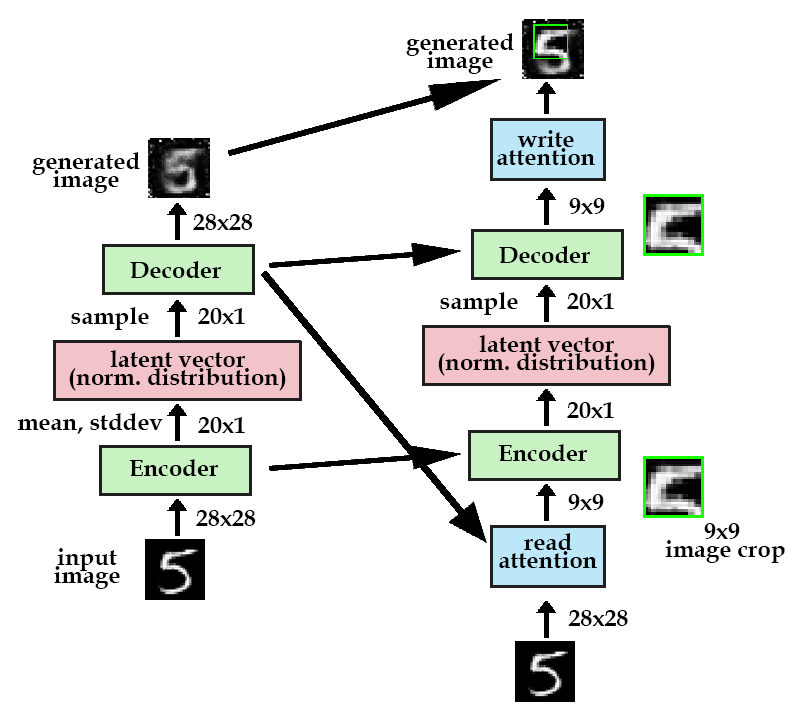
Model with both read and write attention gates. Note that the first timestep should also have read/write attention gates but are omitted for clarity.
To review, the read attention gate takes a 9x9 crop from the 28x28 original image. This crop is then passed through the autoencoder, and the write attention gate places the 9x9 crop at its appropriate position in the 28x28 generated image. This process is then repeated for a number of timesteps until the original image is recreated.
Actually, not really.
Describing the attention mechanism as a crop makes sense intuitively. However, in practice, we use a different method. The model structure described above is still accurate, but we use a matrix of gaussian filters instead of a crop.
What is a gaussian filter? Imagine that our attention gate consisted of taking a 9x9 crop of the original image, and storing the average grayscale value. Then, when reconstructing the image, the a 9x9 patch of that average grayscale value in added on.
A gaussian filter does essentially that, except instead of taking a mean average of the 9x9 area, more influence is placed on the grayscale values near the center.
To gain a better understanding, let's think in one dimension first.
Let's say we had a vector of 10 random values, say [3,5,2,7,4,9,4,6,1,8].
To find the mean average, we would multiply each value by 0.1, and the sum them up.
However, another way to do this is by multiplying each value by its corresponding frequency in a gaussian (otherwise known as normal) distribution, and summing those values up.
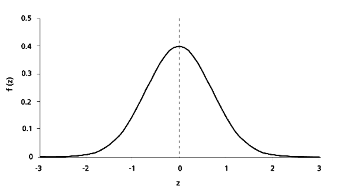
Gaussian/normal distribution [source]
This would place more of an emphasis on the center values such as 4 and 9, and less on the outer values such as 3 and 8.
Furthermore, we can choose the center and spread of our gaussian filter. If we place our filter near the side, values near that area will have more influence.
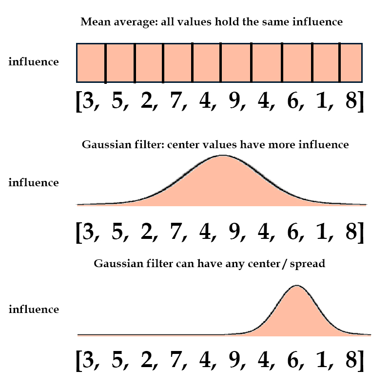
It's important to note that every single value still has some influence, even though it may be tiny. This allows us to pass gradients through the attention gate so we can run backprop.
We can extend this into two dimensions by having two gaussian filters, one along the X axis and one along the Y axis.
To bring it all together: in the previous section we went over a "read" attention gate that chose a center x, center y, and scale for a crop of the original image.
We can use those same parameters to define a gaussian filter. The center x and y will determine at what location in the original image to place the filter, and the scale will determine how much influence is spread out or concentrated.
However, in the end our gaussian filter only leaves us with one scalar average of a certain portion. Ideally, we would want more information than that.
In DRAW, we take an array of gaussian filters, each with their centers spaced apart evenly. For example, we may have a 3x3 array of gaussian filters, with the position of the entire array parameterized by with center x and center y.
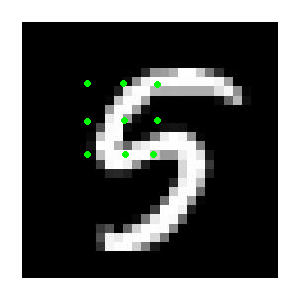
green dots = center of a gaussian filter. X,y coordinates of the center dot are determined by the attention gate.
To account for multiple filte, we need a fourth parameter in our attention gate: stride, or how far apart each filter should be from one another.
These multiple filters allow us to capture 3x3 = 9 values of information during each timestep, instead of only one.
Finally, just for fun we can consider an extreme situation. If we had 28x28 gaussian filters with a stride of one, and each filter had a spread so small it was only influenced by its center pixel, our attention gate would essentially capture the entire original image.
How well does it work?
I ran some experiments on generating the MNIST dataset using an implementation of DRAW in tensorflow.
First, let's look at the plain recurrent version without any attention. The image starts out like a gray blob, and every frame, it gets a little clearer.
DRAW without attention
Here's the fun part. With attention, the image creation gets a bit crazier.
DRAW with attention
It's kind of hard to tell what the network is doing. While it's not exactly the brushstroke-like drawing behavior we were expecting, at the later timesteps you can see that the network only edits a portion of the image at a time.
A thing to note is at the first timestep, the network pays attention to the entire image. Whether this is to create the black background, or to understand what number to draw, is hard to know.
Interestingly, there's actually signs of the network changing its mind about what number to draw. Take a look at the second to last row, fourth from the left. The network starts out by drawing the outline of a 4. However, it goes back and changes that 4 into a 7 midway.
The code for these results is on my Github, which is a slightly fancier and commented version of ericjang's implementation.