The problem with the methods covered earlier is that it requires a model. Oftentimes, the agent does not know how the environment works and must figure it out by themselves.
Model-free prediction is predicting the value function of a certain policy without a concrete model.
The simplest method is Monte-Carlo learning. However, it only works on episodic tasks: where you have a certain set of actions, the the episode ends with some total reward. Monte-Carlo learning states that the return of a state is simply the mean average of the total reward from when a state appeared onwards.
In short, once an episode has concluded, every state that was present can update its value function towards that end return.
However, a problem lies in that every state updates towards the end return, even though that individual state may have had no impact whatsoever on how much reward there was at the end. In order to reduce the variance, we can use a different method of prediction.
Temporal-difference learning, or TD learning, updates the values of each state based on a prediction of the final return. For example, let's say Monte-Carlo learning takes 100 actions and then updates them all based on the final return. TD learning would take an action, and then update the value of the previous action based on the value of the current action. TD learning has the advantage of updating values on more recent trends, in order to capture more of the effect of a certain state.
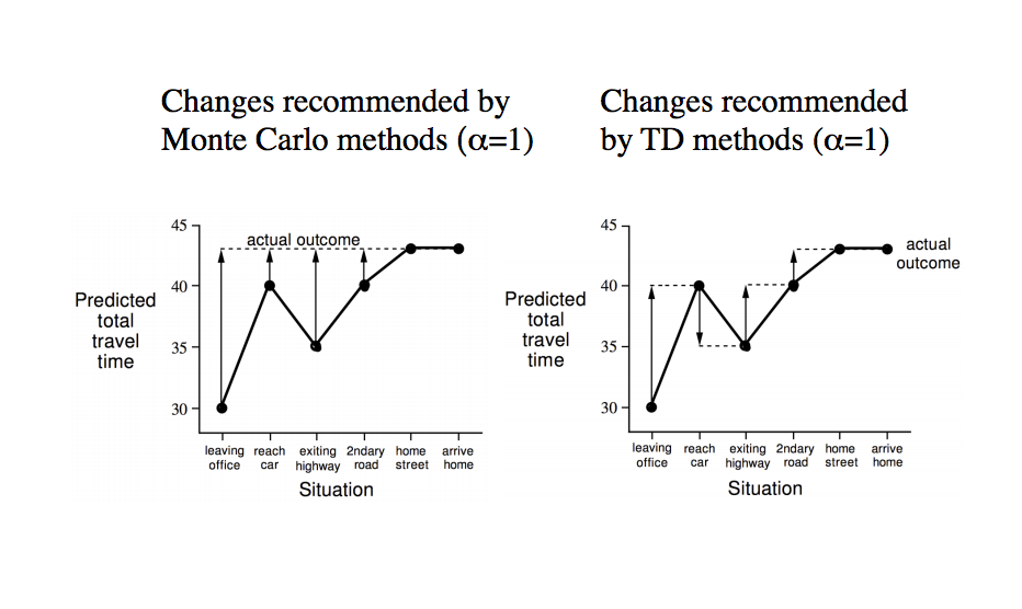
TD has a lower variance than Monte-Carlo, as each update depends on less factors. However, Monte-Carlo has no bias, as values are updated directly towards the final return, while TD has some bias as values are updated towards a prediction.
TD and Monte-Carlo are actually opposite ends of a spectrum between full lookahead and one-step lookahead. Any number of steps can be taken before passing the return back to an action. One step would be the previously discussed TD learning, and infinite steps is Monte-Carlo.
The question rises: how many steps is optimal to look ahead? Unfortunately, it varies greatly depending on the environment and is often a hyperparameter. Another solution is TD(λ), which takes a geometric-weighted average of all n-step lookaheads and uses that to update the value.
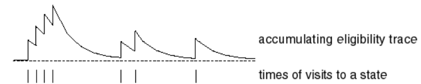
Finally, another way to think about TD(λ) is through eligibility traces. An eligibility trace is some weighting that is assigned to every state, based on how frequently and recently it has shown up. After each action, all states are updated proportionally to their eligibility trace towards the reward.
Model-Free Control
Okay, that's great. We can find value functions for any given policy through experimentation. But how do we improve on this policy to find the optimal strategy?
To do this, we have to return to the idea of policy iteration. Find the value function, change the policy to act greedily towards the value function, and repeat. However, we don't know how the environment works, so the transition probabilities are unknown. We can't act greedily towards state values if we don't know which actions lead to which states!
The solution here is to learn action-values instead of state-values. For every Q(state,action), there is a value corresponding to the expected return of taking a certain action from a certain state. By learning these instead, we can act greedily by simply taking the action with the highest expected return when at a state.
So we've got a basic iteration going, and it works well for simple policies. However, there's a problem with the lack of exploration. Let's say we're at a state with two doors. One door gives a reward of +1 every time, and the other door gives +0 reward, but has a 10% chance to give a reward of +100. On the first run, the second door doesn't get lucky and returns a reward of 0. Since it's acting greedily, the AI will only ever take the first door since it considers it the better option.
How do we fix this? Random exploration. At some probability, the program will take a random action instead of taking the optimal action. This allows it to eventually figure out that there is some extremely high reward hidden behind the second door if it tries it out. However, we want the AI to eventually converge at some optimal policy, so we lower the probability of taking a random action over time.
Finally, we can make use of the same techniques in model-free prediction for control. Eligibility traces work just as well in action-value iteration as in state-iteration.
There's also a little bit about learning off-policy, or learning by watching another policy make decisions. We can utilize a method named Q-learning, which is an update very similar to our random exploration. The value of Q(state,action) is updated towards the reward of an some arbitrary action that the observed policy decides on, and the expected return from that state onwards according to our greedy policy. Basically, we watch what the other policy did and how it affected the environment, and assess how good the move was depending on out current action-values.
More information about the difference between random-exploration (SARSA) and Q-learning: https://studywolf.wordpress.com/2013/07/01/reinforcement-learning-sarsa-vs-q-learning/
Approximating the Value Function
The methods we've been using in reinforcement learning often make use of a value function, either based on states or actions. We've been assuming some concrete mapping of states to values, such as a table. However, in some problems, there may be millions of states. In the case of some real-world problems such as controlling a robot arm, there may be almost infinite states for each joint.
Therefore, for most practical applications it is useful to use a function approximator to estimate the value function given a state. This can be anything from a neural network to just some linear combination of features.
Let's take a standard policy evaluation algorithm, using TD. Instead of updating the value of a table on every iteration, we can make a supervised training call to a neural network that takes in Markov states as input and outputs the value of that state. If we're doing control, the action can be encoded as a one-hot vector and included in the network input. For TD(λ), eligibility traces can be stored on individual features of the Markov state to produce the same effect.
However, there are some downsides to using a neural network as a value function. Since we're updating the network on values that are bootstrapped off its own output (in the case of TD), the network might never converge and instead scale up to infinity or down to 0.
There are two tricks that can help combat this. Instead of training the network on the current TD value, we instead save that "experience" into some array. We then train the network on a batch of randomly selected experiences from the past. This not only decreases correlation, but allows us to reuse data to make training more efficient.
We also hold two copies of the neural network. One is frozen and does not change, and we bootstrap off of it when calculating TD error. After ~1000 steps or so, we update the frozen neural network with the one we have been training on. This stabilizes the networks and helps prevent the networks from scaling up to infinity.
Note: this is a continuation from a previous post, with information taken from David Silver's RL Course.